We’ve discussed at some length what happens if we start from axioms and then build up an “entailment cone” of all statements that can be derived from them. But in the actual practice of mathematics people often want to just look at particular target statements, and see if they can be derived (i.e. proved) from the axioms.
But what can we say “in bulk” about this process? The best source of potential examples we have right now come from the practice of automated theorem proving—as for example implemented in the Wolfram Language function FindEquationalProof. As a simple example of how this works, consider the axiom
and the theorem:
Automated theorem proving (based on FindEquationalProof) finds the following proof of this theorem:
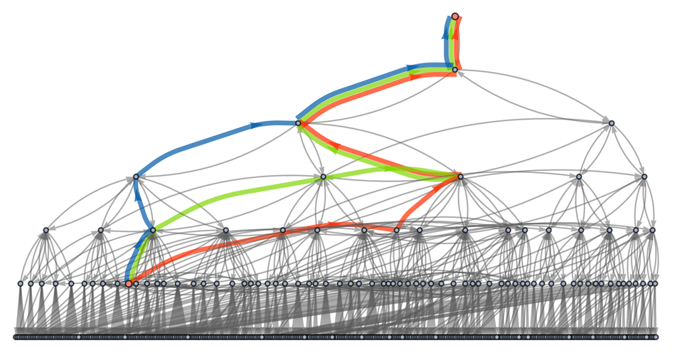
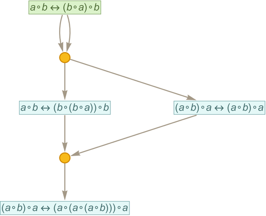
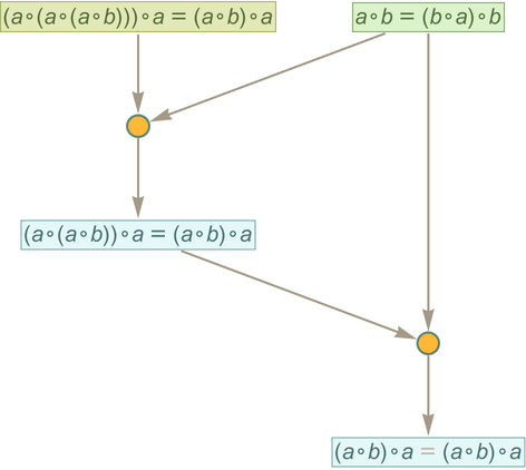
Needless to say, this isn’t the only possible proof. And in this very simple case, we can construct the full entailment cone—and determine that there aren’t any shorter proofs, though there are two more of the same length:
All three of these proofs can be seen as paths in the entailment cone:
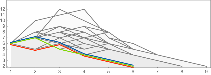
How “complicated” are these proofs? In addition to their lengths, we can for example ask how big the successive intermediate expressions they involve become, where here we are including not only the proofs already shown, but also some longer ones as well:
In the setup we’re using here, we can find a proof of lhs rhs by starting with lhs, building up an entailment cone, and seeing whether there’s any path in it that reaches rhs. In general there’s no upper bound on how far one will have to go to find such a path—or how big the intermediate expressions may need to get.
One can imagine all kinds of optimizations, for example where one looks at multistep consequences of the original axioms, and treats these as “lemmas” that we can “add as axioms” to provide new rules that jump multiple steps on a path at a time. Needless to say, there are lots of tradeoffs in doing this. (Is it worth the memory to store the lemmas? Might we “jump” past our target? etc.)
But typical actual automated theorem provers tend to work in a way that is much closer to our accumulative rewriting systems—in which the “raw material” on which one operates is statements rather than expressions.
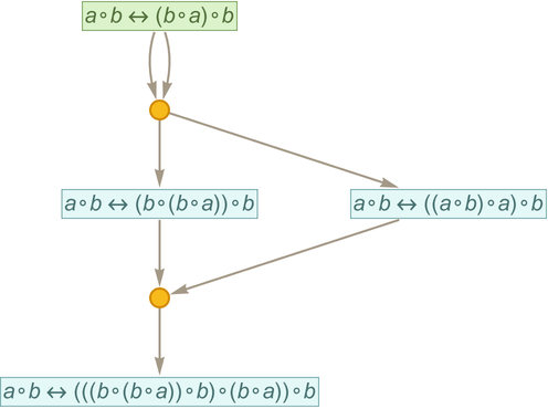
Once again, we can in principle always construct a whole entailment cone, and then look to see whether a particular statement occurs there. But then to give a proof of that statement it’s sufficient to find the subgraph of the entailment cone that leads to that statement. For example, starting with the axiom
we get the entailment cone (shown here as a token-event graph, and dropping _’s):
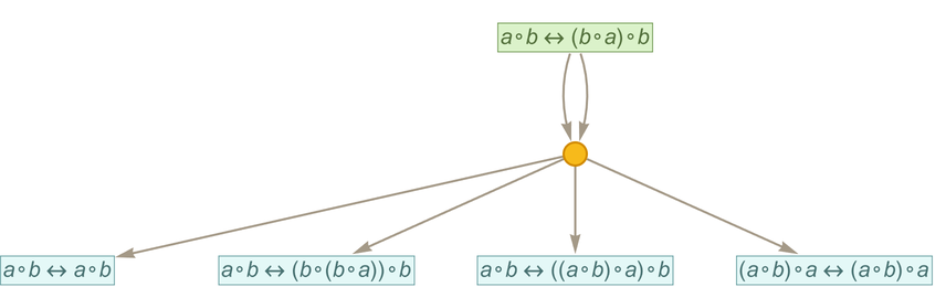
After 2 steps the statement
shows up in this entailment cone
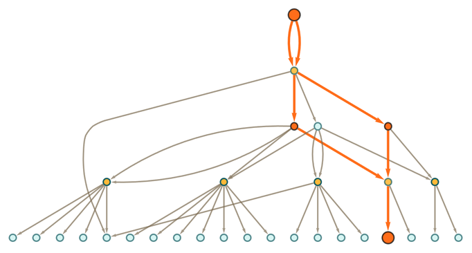
where we’re indicating the subgraph that leads from the original axiom to this statement. Extracting this subgraph we get
which we can view as a proof of the statement within this axiom system.
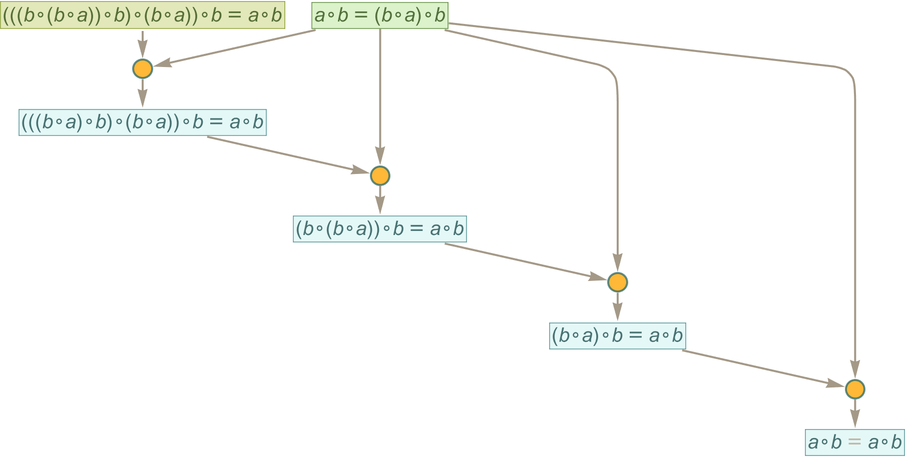
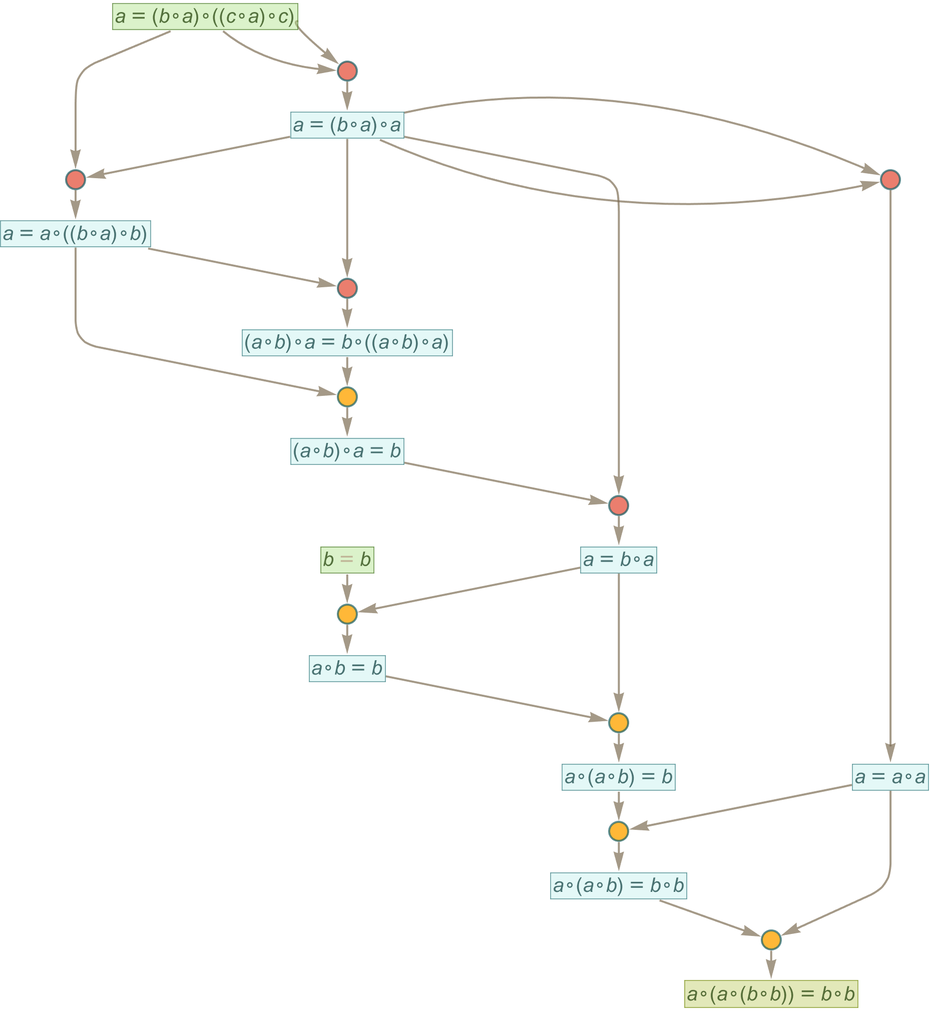
But now let’s use traditional automated theorem proving (in the form of FindEquationalProof) to get a proof of this same statement. Here’s what we get:
This is again a token-event graph, but its structure is slightly different from the one we “fished out of” the entailment cone. Instead of starting from the axiom and “progressively deriving” our statement we start from both the statement and the axiom and then show that together they lead “merely via substitution” to a statement of the form x=x, which we can take as an “obviously derivable tautology”.
Sometimes the minimal “direct proof” found from the entailment cone can be considerably simpler than the one found by automated theorem proving. For example, for the statement
the minimal direct proof is
while the one found by FindEquationalProof is:
But the great advantage of automated theorem proving is that it can “directedly” search for proofs instead of just “fishing them out of” the entailment cone that contains all possible exhaustively generated proofs. To use automated theorem proving you have to “know where you want to go”—and in particular identify the theorem you want to prove.
Consider the axiom
and the statement:
This statement doesn’t show up in the first few steps of the entailment cone for the axiom, even though millions of other theorems do. But automated theorem proving finds a proof of it—and rearranging the “prove-a-tautology proof” so that we just have to feed in a tautology somewhere in the proof, we get:
The model-theoretic methods we’ll discuss a little later allow one effectively to “guess” theorems that might be derivable from a given axiom system. So, for example, for the axiom system
here's a “guess” at a theorem
and here’s a representation of its proof found by automated theorem proving—where now the length of an intermediate “lemma” is indicated by the size of the corresponding node
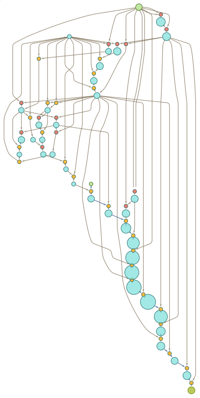
and in this case the longest intermediate lemma is of size 67 and is:
In principle it’s possible to rearrange token-event graphs generated by automated theorem proving to have the same structure as the ones we get directly from the entailment cone—with axioms at the beginning and the theorem being proved at the end. But typical strategies for automated theorem proving don’t naturally produce such graphs. In principle automated theorem proving could work by directly searching for a “path” that leads to the theorem one’s trying to prove. But usually it’s much easier instead to have as the “target” a simple tautology.
At least conceptually automated theorem proving must still try to “navigate” through the full token-event graph that makes up the entailment cone. And the main issue in doing this is that there are many places where one does not know “which branch to take”. But here there’s a crucial—if at first surprising—fact: at least so long as one is using full bisubstitution it ultimately doesn’t matter which branch one takes; there’ll always be a way to “merge back” to any other branch.
This is a consequence of the fact that the accumulative systems we’re using automatically have the property of confluence which says that every branch is accompanied by a subsequent merge. There’s an almost trivial way in which this is true by virtue of the fact that for every edge the system also includes the reverse of that edge. But there’s a more substantial reason as well: that given any two statements on two different branches, there’s always a way to combine them using a bisubstitution to get a single statement.
In our Physics Project, the concept of causal invariance—which effectively generalizes confluence—is an important one, that leads among other things to ideas like relativistic invariance. Later on we’ll discuss the idea that “regardless of what order you prove theorems in, you’ll always get the same math”, and its relationship to causal invariance and to the notion of relativity in metamathematics. But for now the importance of confluence is that it has the potential to simplify automated theorem proving—because in effect it says one can never ultimately “make a wrong turn” in getting to a particular theorem, or, alternatively, that if one keeps going long enough every path one might take will eventually be able to reach every theorem.
And indeed this is exactly how things work in the full entailment cone. But the challenge in automated theorem proving is to generate only a tiny part of the entailment cone, yet still “get to” the theorem we want. And in doing this we have to carefully choose which “branches” we should try to merge using bisubstitution events. In automated theorem proving these bisubstitution events are typically called “critical pair lemmas”, and there are a variety of strategies for defining an order in which critical pair lemmas should be tried.
It’s worth pointing out that there’s absolutely no guarantee that such procedures will find the shortest proof of any given theorem (or in fact that they’ll find a proof at all with a given amount of computational effort). One can imagine “higher-order proofs” in which one attempts to transform not just statements of the form lhsrhs, but full proofs (say represented as token-event graphs). And one can imagine using such transformations to try to simplify proofs.
A general feature of the proofs we’ve been showing is that they are accumulative, in the sense they continually introduce lemmas which are then reused. But in principle any proof can be “unrolled” into one that just repeatedly uses the original axioms (and in fact, purely by substitution)—and never introduces other lemmas. The necessary “cut elimination” can effectively be done by always recreating each lemma from the axioms whenever it’s needed—a process which can become exponentially complex.
As an example, from the axiom above we can generate the proof
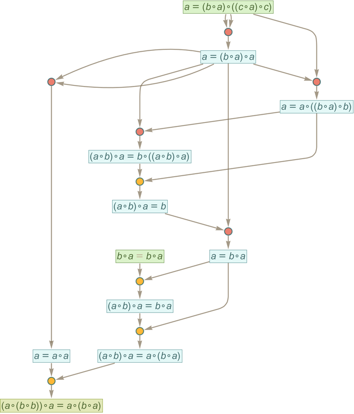
where for example the first lemma at the top is reused in four events. But now by cut elimination we can “unroll” this whole proof into a “straight-line” sequence of substitutions on expressions done just using the original axiom
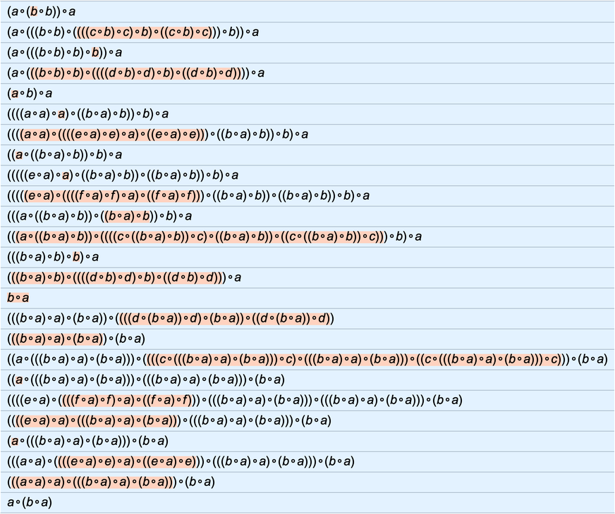
and we see that our final theorem is the statement that the first expression in the sequence is equivalent under the axiom to the last one.
As is fairly evident in this example, a feature of automated theorem proving is that its result tends to be very “non-human”. Yes, it can provide incontrovertible evidence that a theorem is valid. But that evidence is typically far away from being any kind of “narrative” suitable for human consumption. In the analogy to molecular dynamics, an automated proof gives detailed “turn-by-turn instructions” that show how a molecule can reach a certain place in a gas. Typical “human-style” mathematics, on the other hand, operates on a higher level, analogous to talking about overall motion in a fluid. And a core part of what's achieved by our physicalization of metamathematics is understanding why it's possible for mathematical observers like us to perceive mathematics as operating at this higher level.