We’ve discussed the overall structure of metamathematical space, and the general kind of sampling that we humans do of it (as “mathematical observers”) when we do mathematics. But what can we learn from the specifics of human mathematics, and the actual mathematical statements that humans have published over the centuries?
We might imagine that these statements are just ones that—as “accidents of history”—humans have “happened to find interesting”. But there’s definitely more to it—and potentially what’s there is a rich source of “empirical data” relevant to our physicalized laws of mathematics, and to what amounts to their “experimental validation”.
The situation with “human settlements” in metamathematical space is in a sense rather similar to the situation with human settlements in physical space. If we look at where humans have chosen to live and build cities, we’ll find a bunch of locations in 3D space. The details of where these are depend on history and many factors. But there’s a clear overarching theme, that’s in a sense a direct reflection of underlying physics: all the locations lie on the more-or-less spherical surface of the Earth.
It’s not so straightforward to see what’s going on in the metamathematical case, not least because any notion of coordinatization seems to be much more complicated for metamathematical space than for physical space. But we can still begin by doing “empirical metamathematics” and asking questions about for example what amounts to where in metamathematical space we humans have so far established ourselves. And as a first example, let’s consider Boolean algebra.
Even to talk about something called “Boolean algebra” we have to be operating at a level far above the raw ruliad—where we’ve already implicitly aggregated vast numbers of emes to form notions of, for example, variables and logical operations.
But once we’re at this level we can “survey” metamathematical space just by enumerating possible symbolic statements that can be created using the operations we’ve set up for Boolean algebra (here And ∧, Or ∨ and Not ![]() ):
):
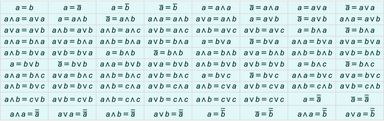
But so far these are just raw, structural statements. To connect with actual Boolean algebra we must pick out which of these can be derived from the axioms of Boolean algebra, or, put another way, which of them are in the entailment cone of these axioms:
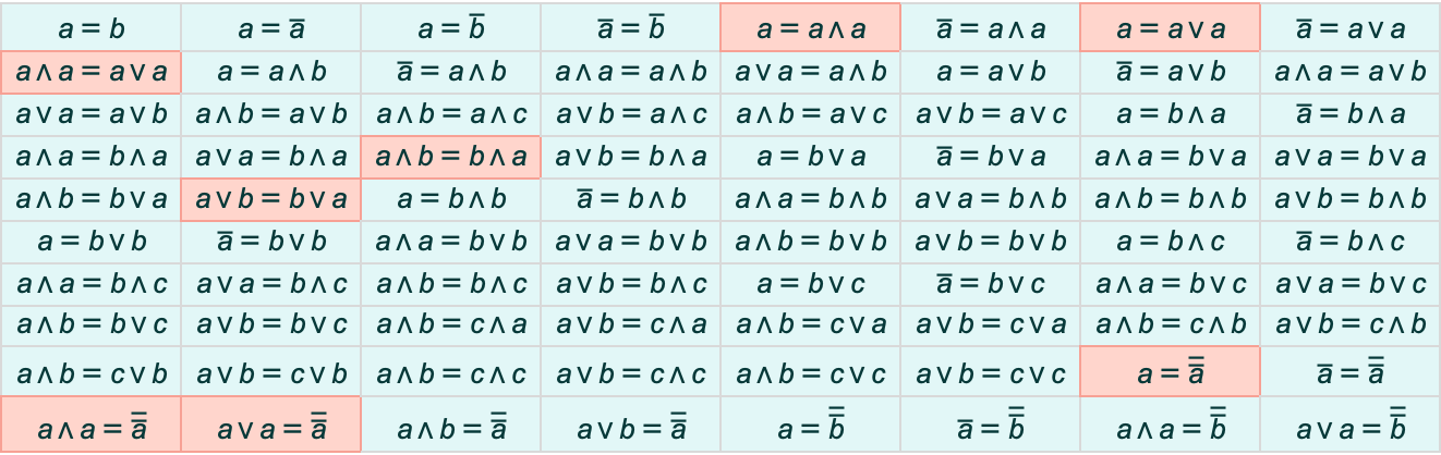
Of all possible statements, it’s only an exponentially small fraction that turn out to be derivable:

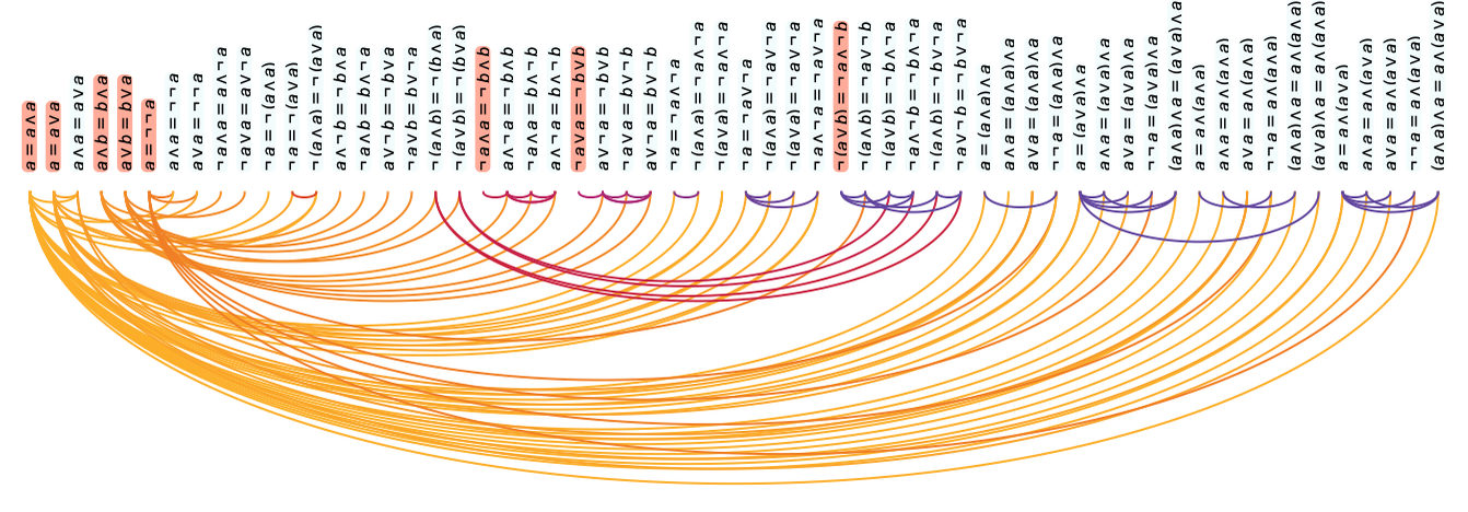
But in the case of Boolean algebra, we can readily collect such statements:
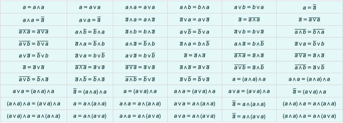
We’ve typically explored entailment cones by looking at slices consisting of collections of theorems generated after a specified number of proof steps. But here we’re making a very different sampling of the entailment cone—looking in effect instead at theorems in order of their structural complexity as symbolic expressions.
In doing this kind of systematic enumeration we’re in a sense operating at a “finer level of granularity” than typical human mathematics. Yes, these are all “true theorems”. But mostly they’re not theorems that a human mathematician would ever write down, or specifically “consider interesting”. And for example only a small fraction of them have historically been given names—and are called out in typical logic textbooks:
The reduction from all “structurally possible” theorems to just “ones we consider interesting” can be thought of as a form of coarse graining. And it could well be that this coarse graining would depend on all sorts of accidents of human mathematical history. But at least in the case of Boolean algebra there seems to be a surprisingly simple and “mechanical” procedure that can reproduce it.
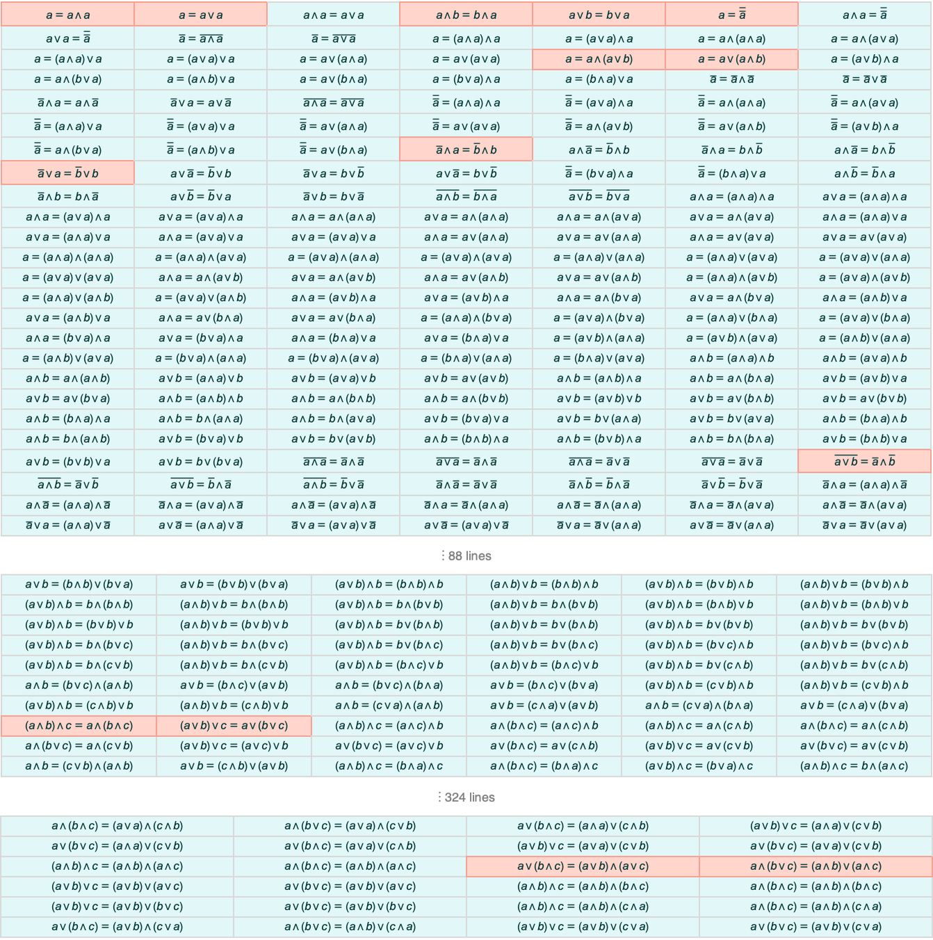
Go through all theorems in order of increasing structural complexity, in each case seeing whether a given theorem can be proved from ones earlier in the list:
It turns out that the theorems identified by humans as “interesting” coincide almost exactly with “root theorems” that cannot be proved from earlier theorems in the list. Or, put another way, the “coarse graining” that human mathematicians do seems (at least in this case) to essentially consist of picking out only those theorems that represent “minimal statements” of new information—and eliding away those that involve “extra ornamentation”.
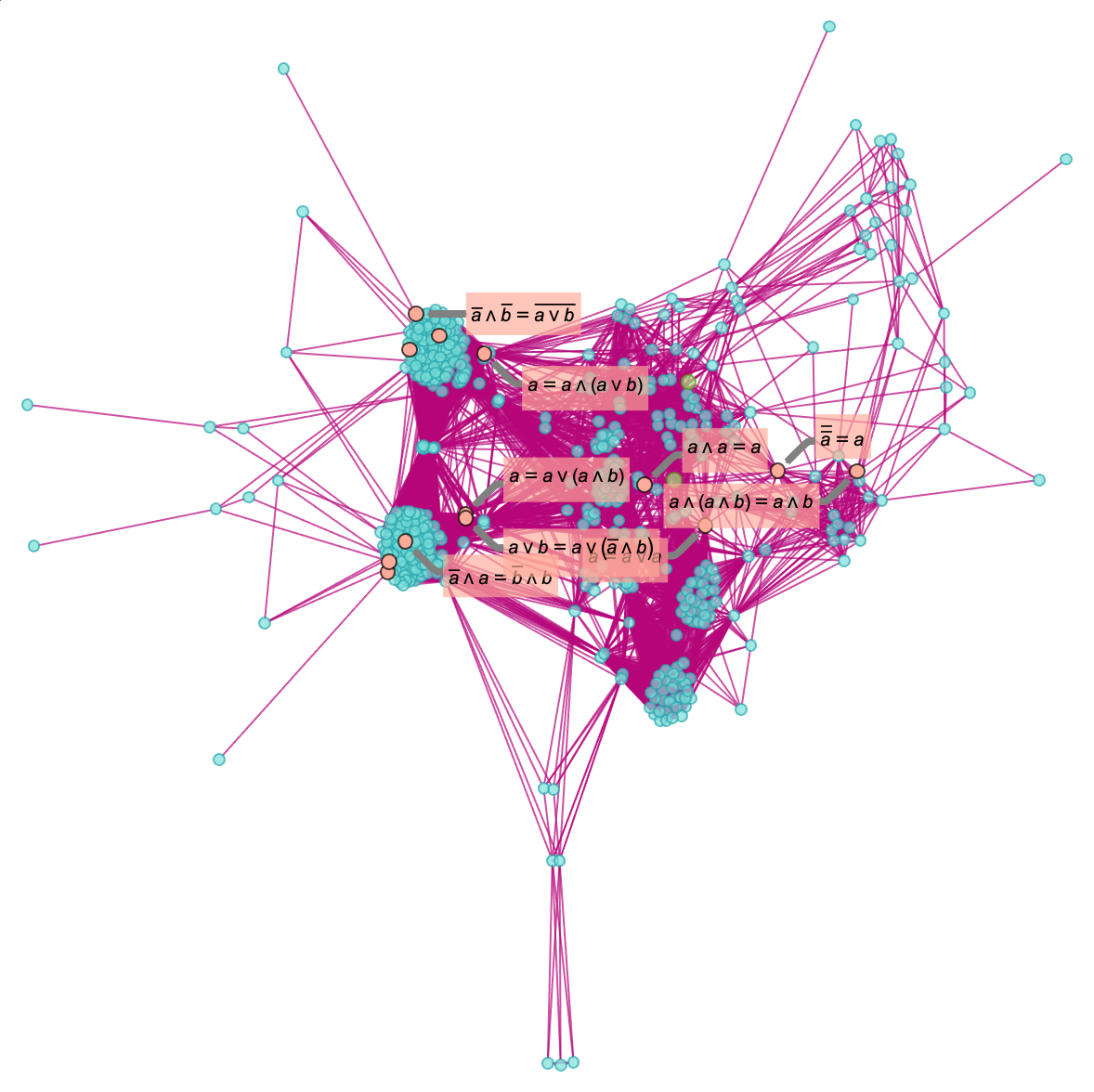
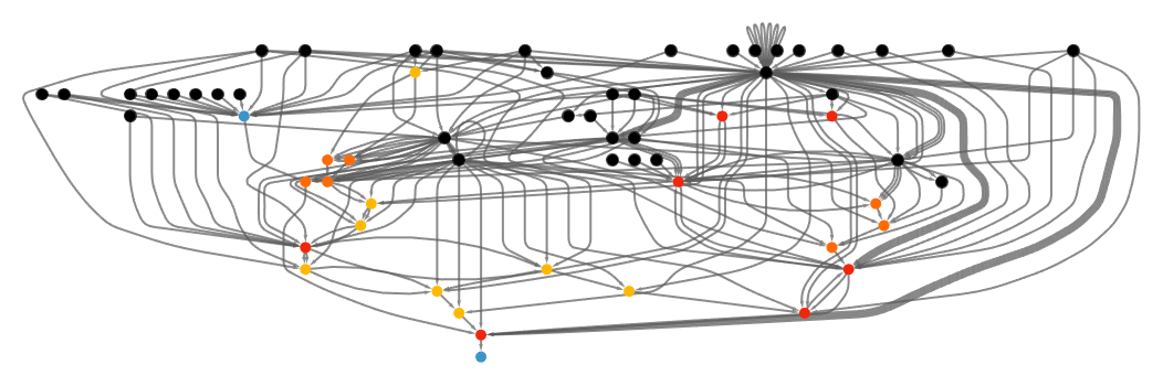
But how are these “notable theorems” laid out in metamathematical space? Earlier we saw how the simplest of them can be reached after just a few steps in the entailment cone of a typical textbook axiom system for Boolean algebra. The full entailment cone rapidly gets unmanageably large but we can get a first approximation to it by generating individual proofs (using automated theorem proving) of our notable theorems, and then seeing how these “knit together” through shared intermediate lemmas in a token-event graph:
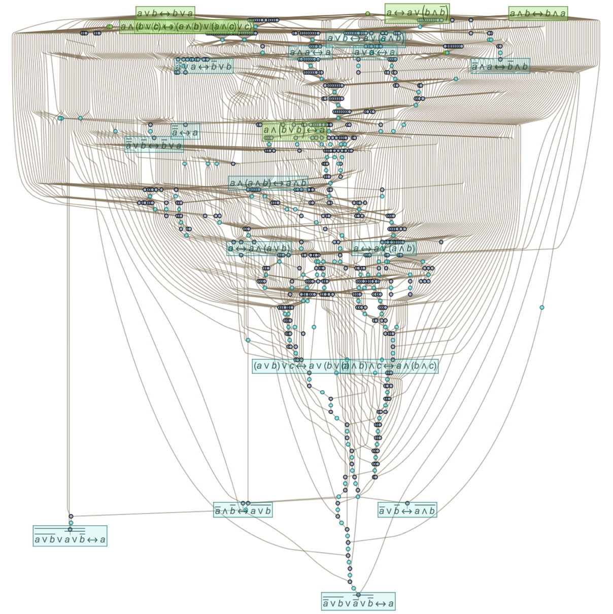
Looking at this picture we see at least a hint that clumps of notable theorems are spread out across the entailment cone, only modestly building on each other—and in effect “staking out separated territories” in the entailment cone. But of the 11 notable theorems shown here, 7 depend on all 6 axioms, while 4 depend only on various different sets of 3 axioms—suggesting at least a certain amount of fundamental interdependence or coherence.
From the token-event graph we can derive a branchial graph that represents a very rough approximation to how the theorems are “laid out in metamathematical space”:
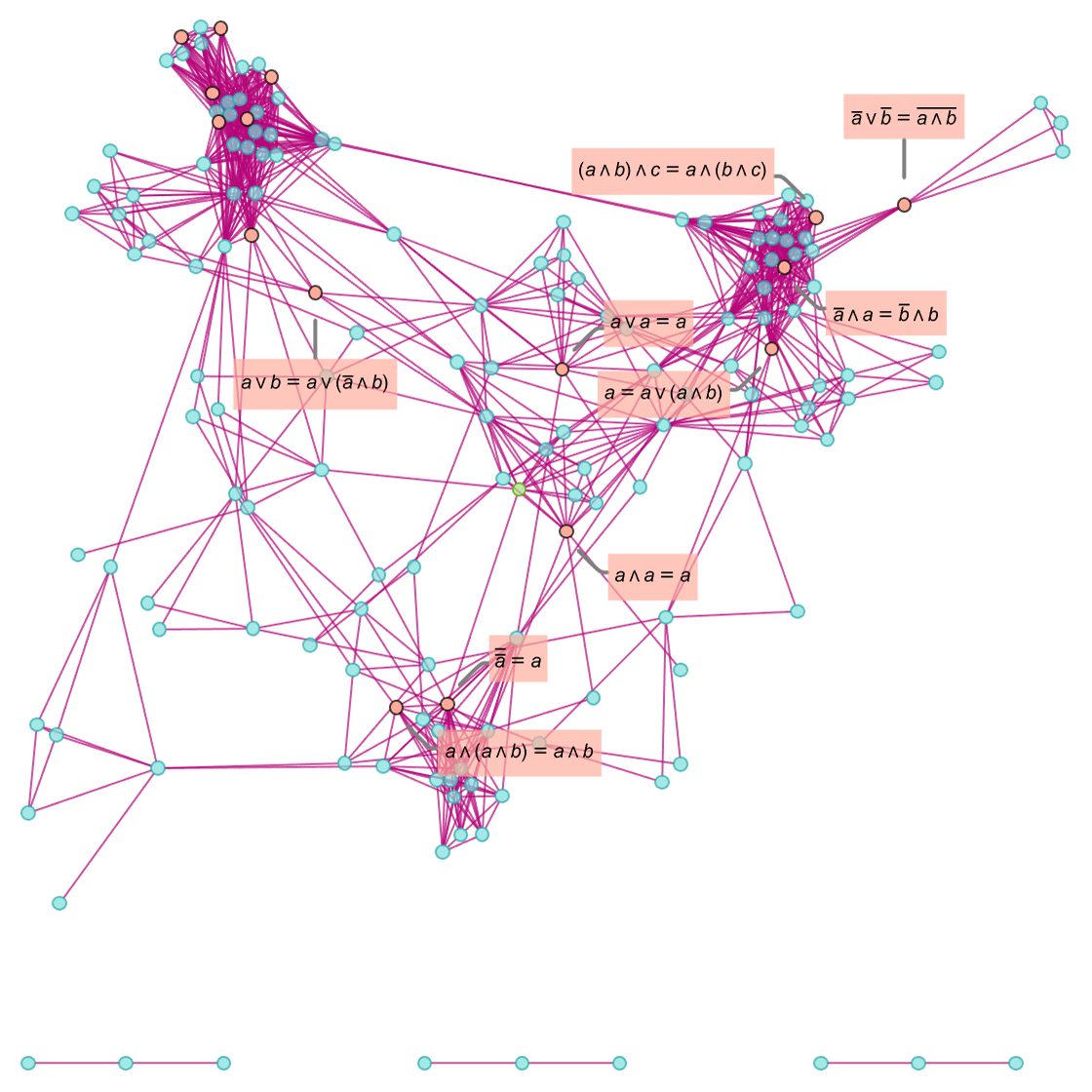
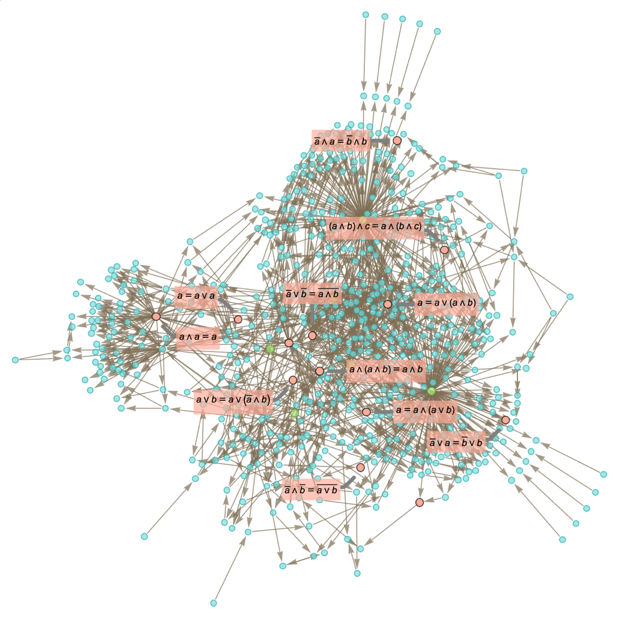
We can get a potentially slightly better approximation by including proofs not just of notable theorems, but of all theorems up to a certain structural complexity. The result shows separation of notable theorems both in the multiway graph
and in the branchial graph:
In doing this empirical metamathematics we’re including only specific proofs rather than enumerating the whole entailment cone. We’re also using only a specific axiom system. And even beyond this, we’re using specific operators to write our statements in Boolean algebra.
In a sense each of these choices represents a particular “metamathematical coordinatization”—or particular reference frame or slice that we’re sampling in the ruliad.
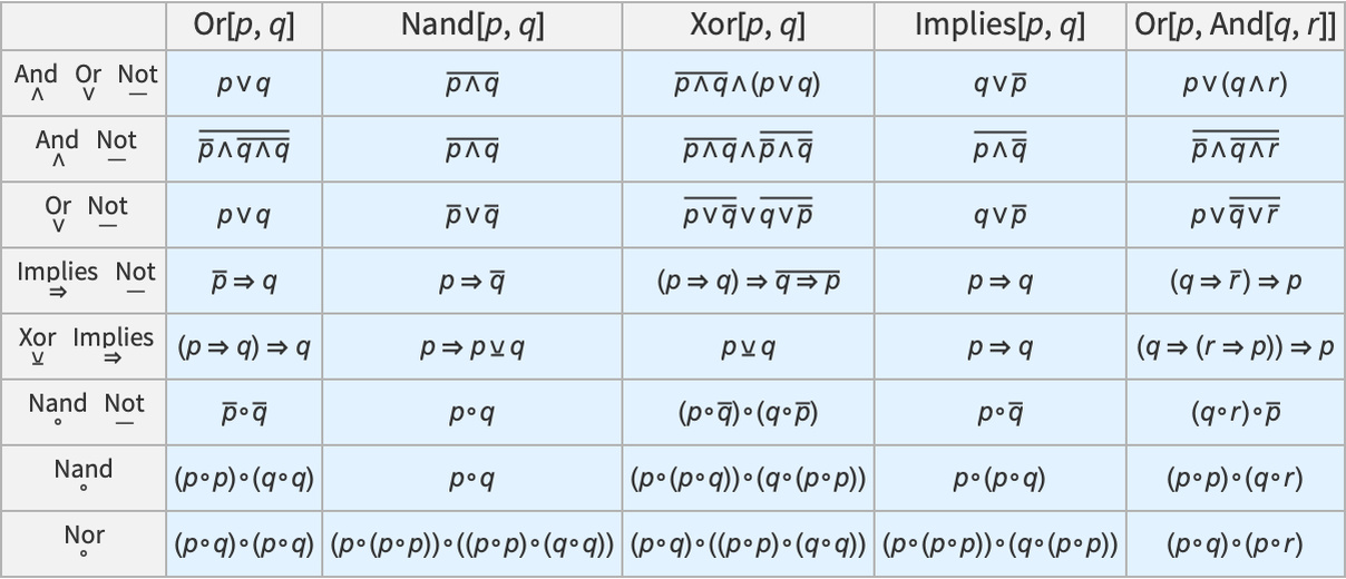
For example, in what we’ve done above we’ve built up statements from And, Or and Not. But we can just as well use any other functionally complete sets of operators, such as the following (here each shown representing a few specific Boolean expressions):
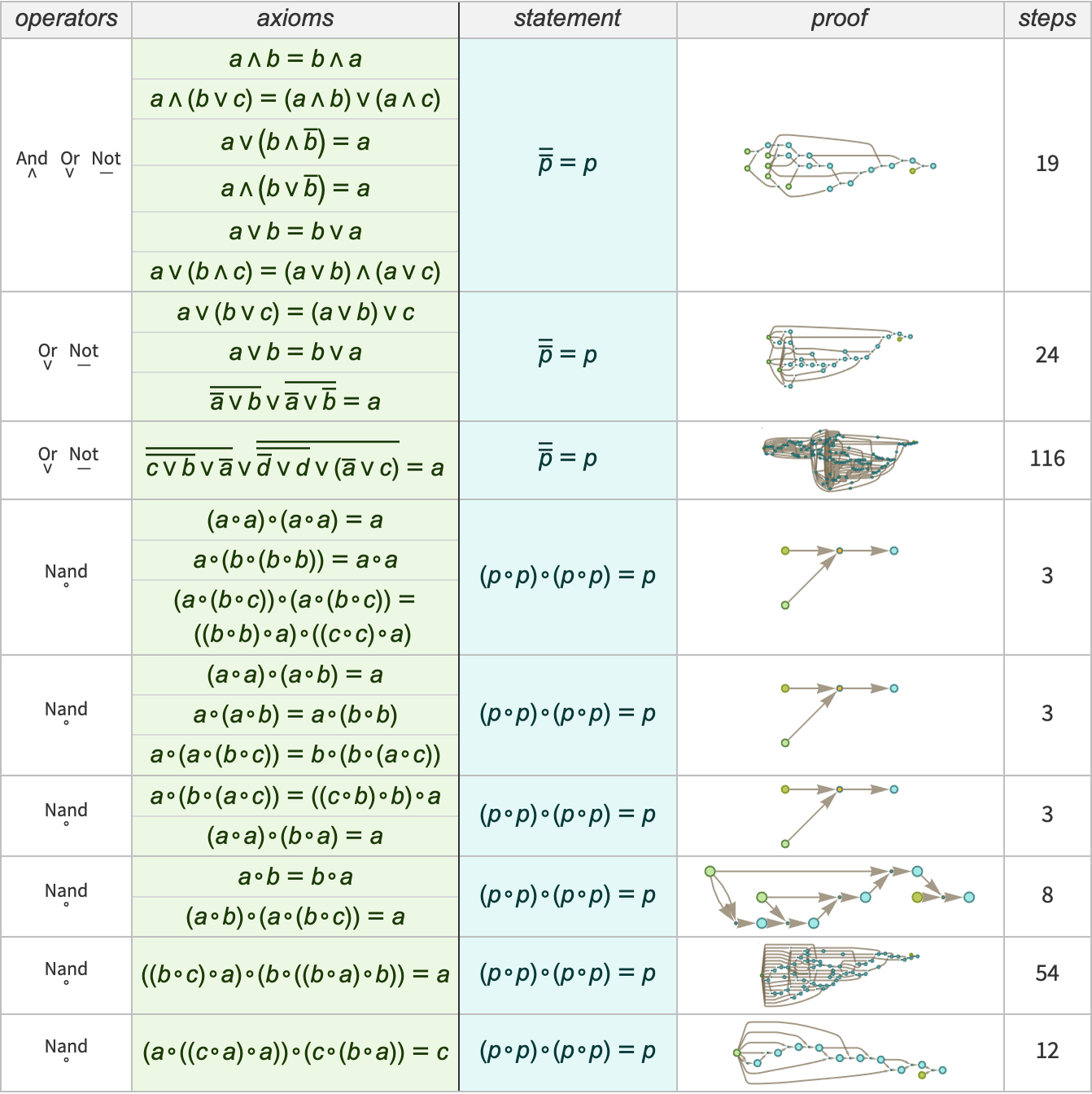
For each set of operators, there are different axiom systems that can be used. And for each axiom system there will be different proofs. Here are a few examples of axiom systems with a few different sets of operators—in each case giving a proof of the law of double negation (which has to be stated differently for different operators):
Boolean algebra (or, equivalently, propositional logic) is a somewhat desiccated and thin example of mathematics. So what do we find if we do empirical metamathematics on other areas?
Let’s talk first about geometry—for which Euclid’s Elements provided the very first large-scale historical example of an axiomatic mathematical system. The Elements started from 10 axioms (5 “postulates” and 5 “common notions”), then gave 465 theorems.
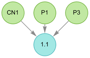
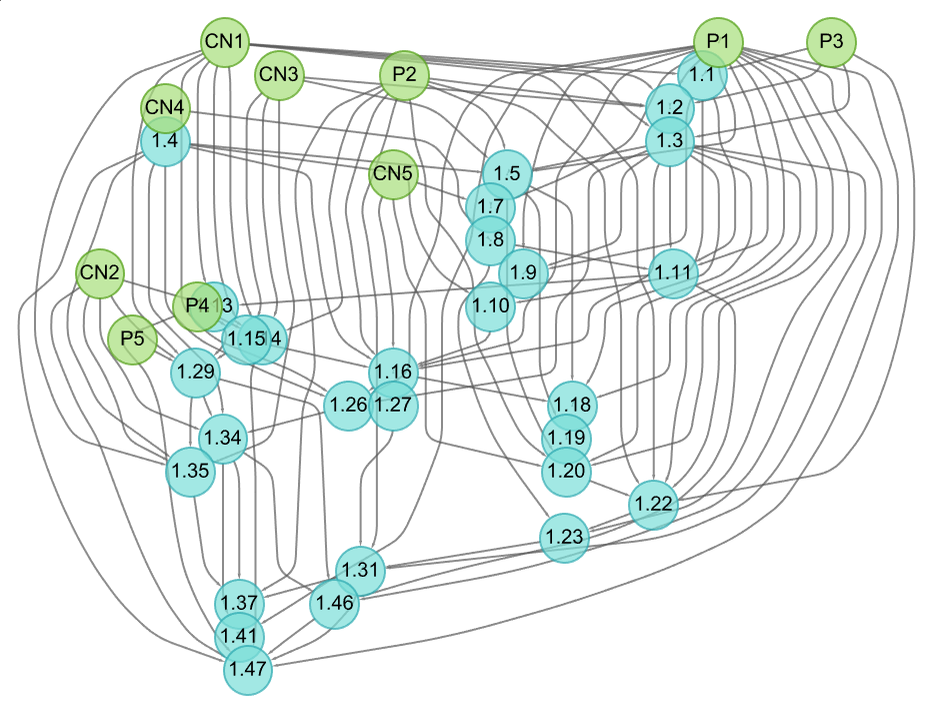
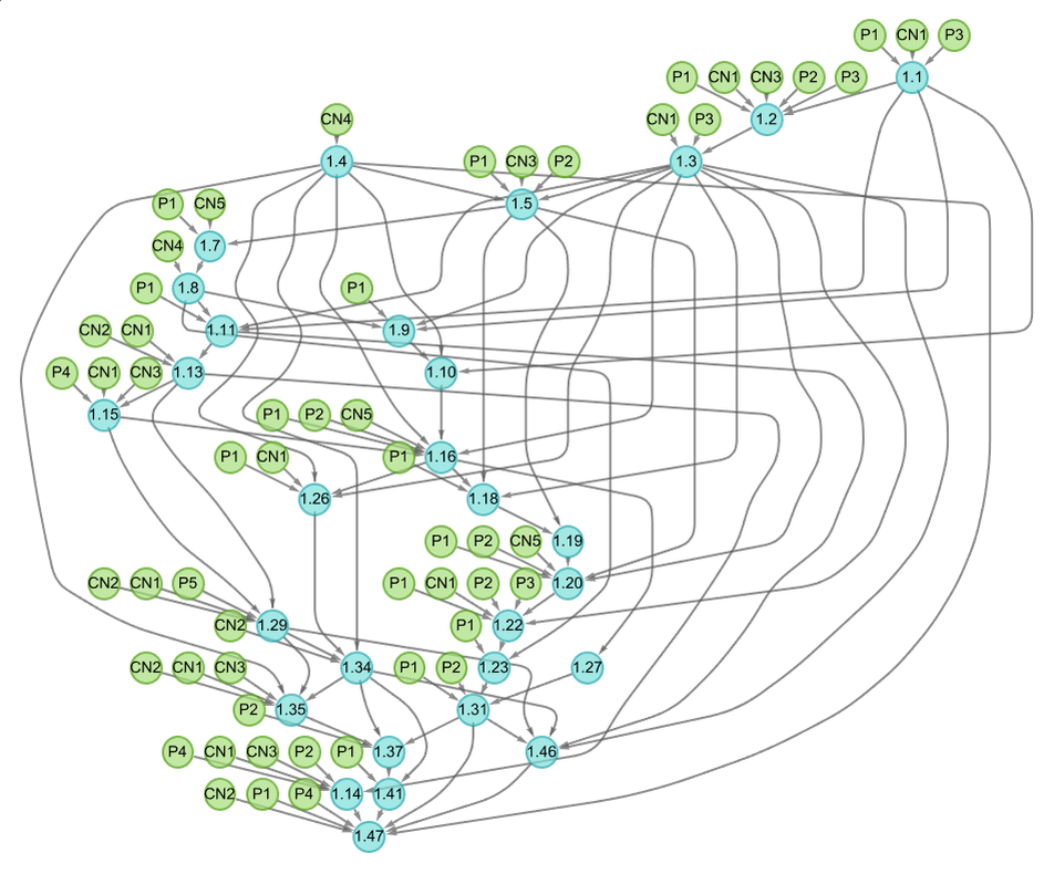
Each theorem was proved from previous ones, and ultimately from the axioms. Thus, for example, the “proof graph” (or “theorem dependency graph”) for Book 1, Proposition 5 (which says that angles at the base of an isosceles triangle are equal) is:
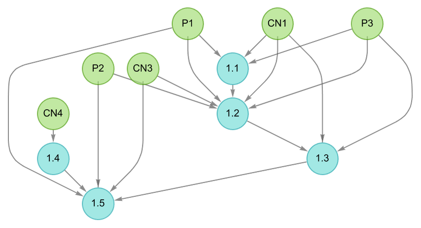
One can think of this as a coarse-grained version of the proof graphs we’ve used before (which are themselves in turn “slices” of the entailment graph)—in which each node shows how a collection of “input” theorems (or axioms) entails a new theorem.
Here’s a slightly more complicated example (Book 1, Proposition 48) that ultimately depends on all 10 of the original axioms:
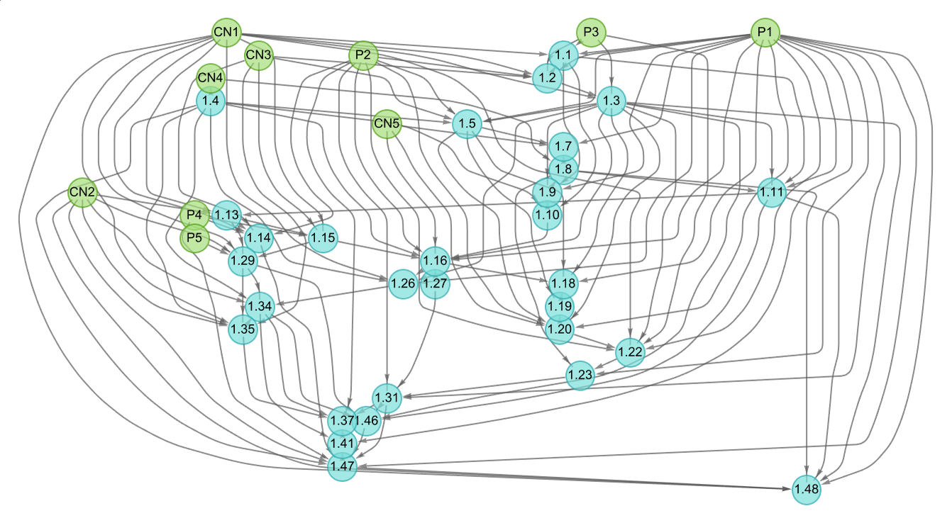
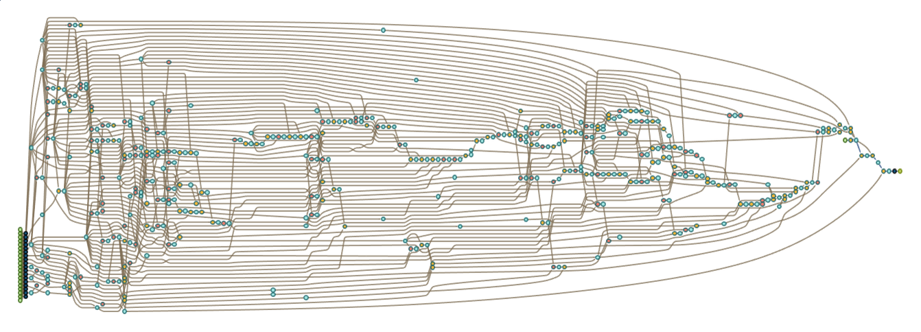
And here’s the full graph for all the theorems in Euclid’s Elements:
Of the 465 theorems here, 255 (i.e. 55%) depend on all 10 axioms. (For the much smaller number of notable theorems of Boolean algebra above we found that 64% depended on all 6 of our stated axioms.) And the general connectedness of this graph in effect reflects the idea that Euclid’s theorems represent a coherent body of connected mathematical knowledge.
The branchial graph gives us an idea of how the theorems are “laid out in metamathematical space”:
One thing we notice is that theorems about different areas—shown here in different colors—tend to be separated in metamathematical space. And in a sense the seeds of this separation are already evident if we look “textually” at how theorems in different books of Euclid’s Elements refer to each other:
Looking at the overall dependence of one theorem on others in effect shows us a very coarse form of entailment. But can we go to a finer level—as we did above for Boolean algebra? As a first step, we have to have an explicit symbolic representation for our theorems. And beyond that, we have to have a formal axiom system that describes possible transformations between these.
At the level of “whole theorem dependency” we can represent the entailment of Euclid’s Book 1, Proposition 1 from axioms as:
But if we now use the full, formal axiom system for geometry that we discussed in a previous section we can use automated theorem proving to get a full proof of Book 1, Proposition 1:
In a sense this is “going inside” the theorem dependency graph to look explicitly at how the dependencies in it work. And in doing this we see that what Euclid might have stated in words in a sentence or two is represented formally in terms of hundreds of detailed intermediate lemmas. (It’s also notable that whereas in Euclid’s version, the theorem depends only on 3 out of 10 axioms, in the formal version the theorem depends on 18 out of 20 axioms.)
How about for other theorems? Here is the theorem dependency graph from Euclid’s Elements for the Pythagorean theorem (which Euclid gives as Book 1, Proposition 47):
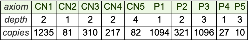
The theorem depends on all 10 axioms, and its stated proof goes through 28 intermediate theorems (i.e. about 6% of all theorems in the Elements). In principle we can “unroll” the proof dependency graph to see directly how the theorem can be “built up” just from copies of the original axioms. Doing a first step of unrolling we get:
And “flattening everything out” so that we don’t use any intermediate lemmas but just go back to the axioms to “re-prove” everything we can derive the theorem from a “proof tree” with the following number of copies of each axiom (and a certain “depth” to reach that axiom):
So how about a more detailed and formal proof? We could certainly in principle construct this using the axiom system we discussed above.
But an important general point is that the thing we in practice call “the Pythagorean theorem” can actually be set up in all sorts of different axiom systems. And as an example let’s consider setting it up in the main actual axiom system that working mathematicians typically imagine they’re (usually implicitly) using, namely ZFC set theory.
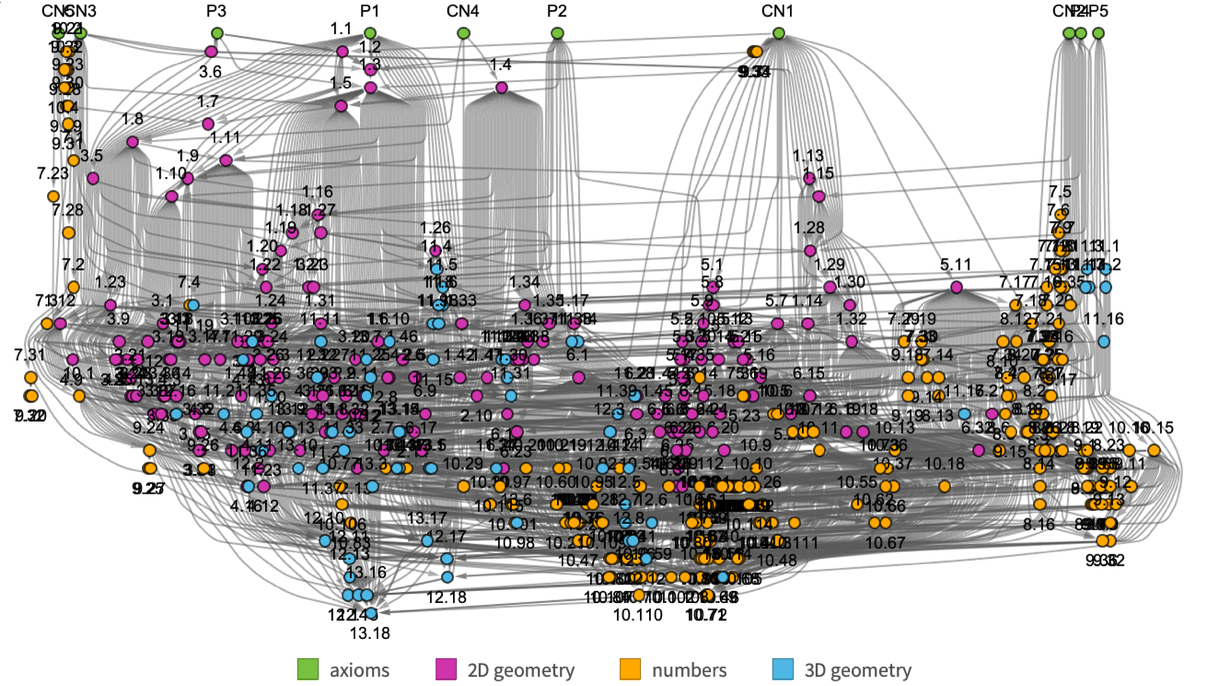
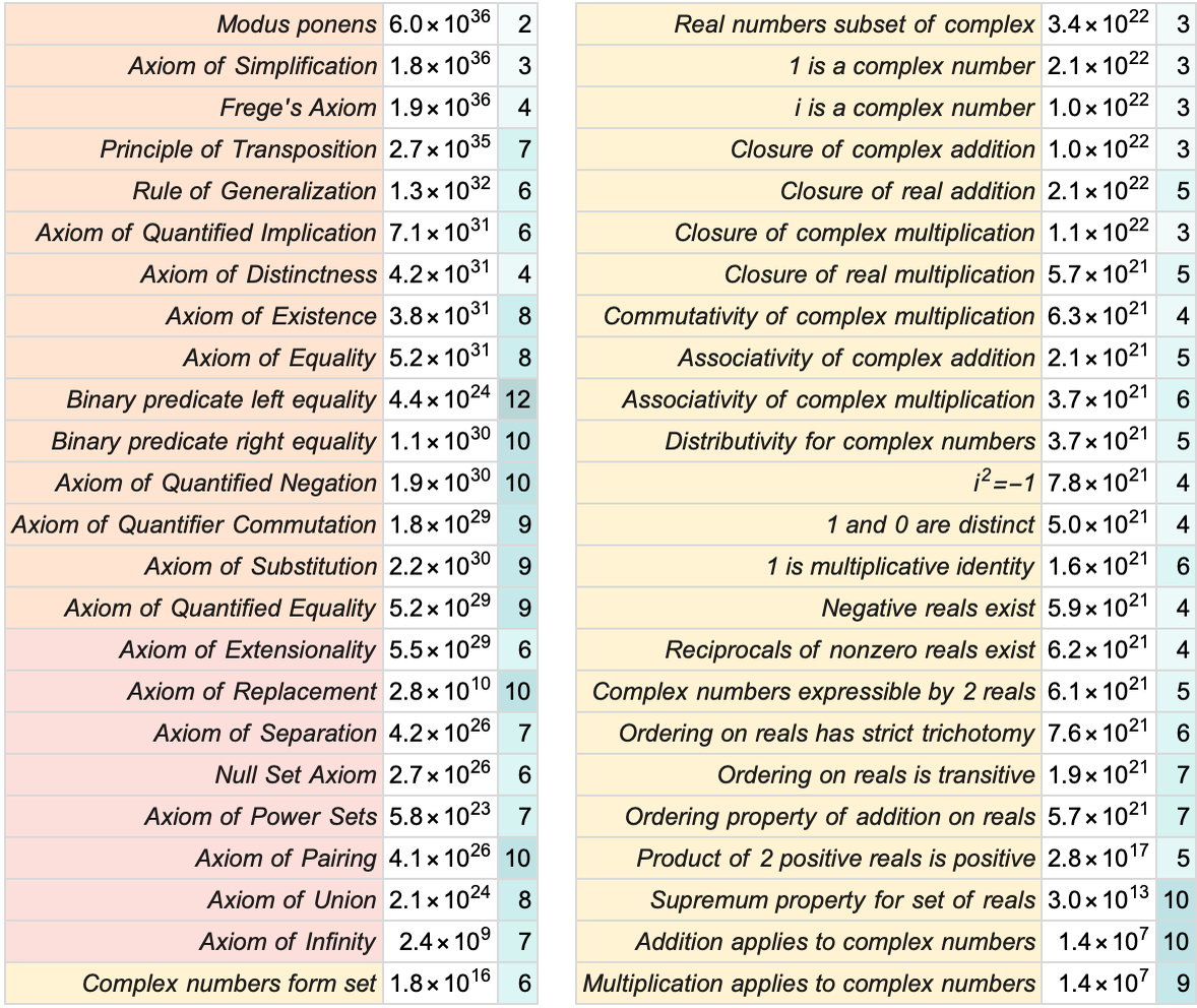
Conveniently, the Metamath formalized math system has accumulated about 40,000 theorems across mathematics, all with hand-constructed proofs based ultimately on ZFC set theory. And within this system we can find the theorem dependency graph for the Pythagorean theorem:
Altogether it involves 6970 intermediate theorems, or about 18% of all theorems in Metamath—including ones from many different areas of mathematics. But how does it ultimately depend on the axioms? First, we need to talk about what the axioms actually are. In addition to “pure ZFC set theory”, we need axioms for (predicate) logic, as well as ones that define real and complex numbers. And the way things are set up in Metamath’s “set.mm” there are (essentially) 49 basic axioms (9 for pure set theory, 15 for logic and 25 related to numbers). And much as in Euclid’s Elements we found that the Pythagorean theorem depended on all the axioms, so now here we find that the Pythagorean theorem depends on 48 of the 49 axioms—with the only missing axiom being the Axiom of Choice.
Just like in the Euclid’s Elements case, we can imagine “unrolling” things to see how many copies of each axiom are used. Here are the results—together with the “depth” to reach each axiom:
And, yes, the numbers of copies of most of the axioms required to establish the Pythagorean theorem are extremely large.
There are several additional wrinkles that we should discuss. First, we’ve so far only considered overall theorem dependency—or in effect “coarse-grained entailment”. But the Metamath system ultimately gives complete proofs in terms of explicit substitutions (or, effectively, bisubstitutions) on symbolic expressions. So, for example, while the first-level “whole-theorem-dependency” graph for the Pythagorean theorem is
the full first-level entailment structure based on the detailed proof is (where the black vertices indicate “internal structural elements” in the proof—such as variables, class specifications and “inputs”):
Another important wrinkle has to do with the concept of definitions. The Pythagorean theorem, for example, refers to squaring numbers. But what is squaring? What are numbers? Ultimately all these things have to be defined in terms of the “raw data structures” we’re using.
In the case of Boolean algebra, for example, we could set things up just using Nand (say denoted ∘), but then we could define And and Or in terms of Nand (say as (p∘q)∘(p∘q) and (p∘p)∘(q∘q) respectively). We could still write expressions using And and Or—but with our definitions we’d immediately be able to convert these to pure Nands. Axioms—say about Nand—give us transformations we can use repeatedly to make derivations. But definitions are transformations we use “just once” (like macro expansion in programming) to reduce things to the point where they involve only constructs that appear in the axioms.
In Metamath’s “set.mm” there are about 1700 definitions that effectively build up from “pure set theory” (as well as logic, structural elements and various axioms about numbers) to give the mathematical constructs one needs. So, for example, here is the definition dependency graph for addition (“+” or Plus):
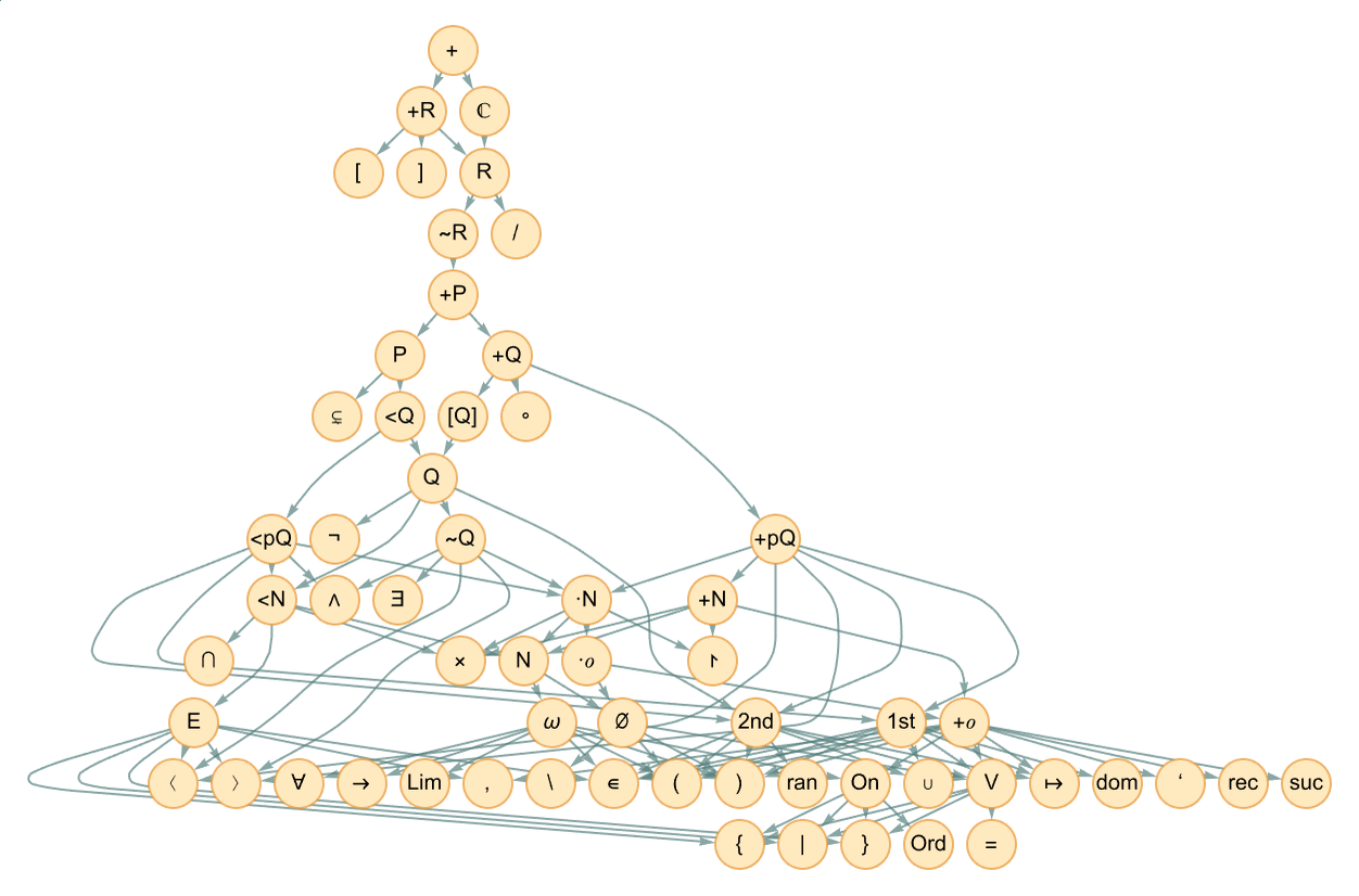
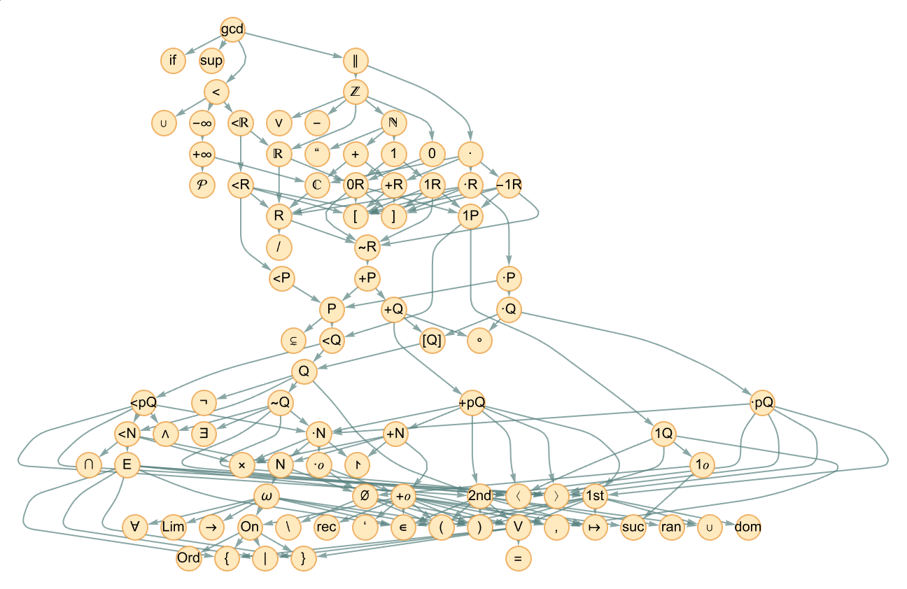
At the bottom are the basic constructs of logic and set theory—in terms of which things like order relations, complex numbers and finally addition are defined. The definition dependency graph for GCD, for example, is somewhat larger, though has considerable overlap at lower levels:
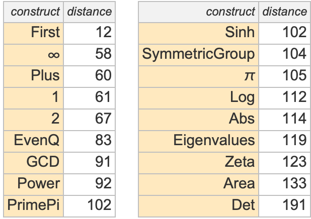
Different constructs have definition dependency graphs of different sizes—in effect reflecting their “definitional distance” from set theory and the underlying axioms being used:
In our physicalized approach to metamathematics, though, something like set theory is not our ultimate foundation. Instead, we imagine that everything is eventually built up from the raw ruliad, and that all the constructs we’re considering are formed from what amount to configurations of emes in the ruliad. We discussed above how constructs like numbers and logic can be obtained from a combinator representation of the ruliad.
We can view the definition dependency graph above as being an empirical example of how somewhat higher-level definitions can be built up. From a computer science perspective, we can think of it as being like a type hierarchy. From a physics perspective, it’s as if we’re starting from atoms, then building up to molecules and beyond.
It’s worth pointing out, however, that even the top of the definition hierarchy in something like Metamath is still operating very much at an axiomatic kind of level. In the analogy we’ve been using, it’s still for the most part “formulating math at the molecular dynamics level” not at the more human “fluid dynamics” level.
We’ve been talking about “the Pythagorean theorem”. But even on the basis of set theory there are many different possible formulations one can give. In Metamath, for example, there is the pythag version (which is what we’ve been using), and there is also a (somewhat more general) pythi version. So how are these related? Here’s their combined theorem dependency graph (or at least the first two levels in it)—with red indicating theorems used only in deriving pythag, blue indicating ones used only in deriving pythi, and purple indicating ones used in both:
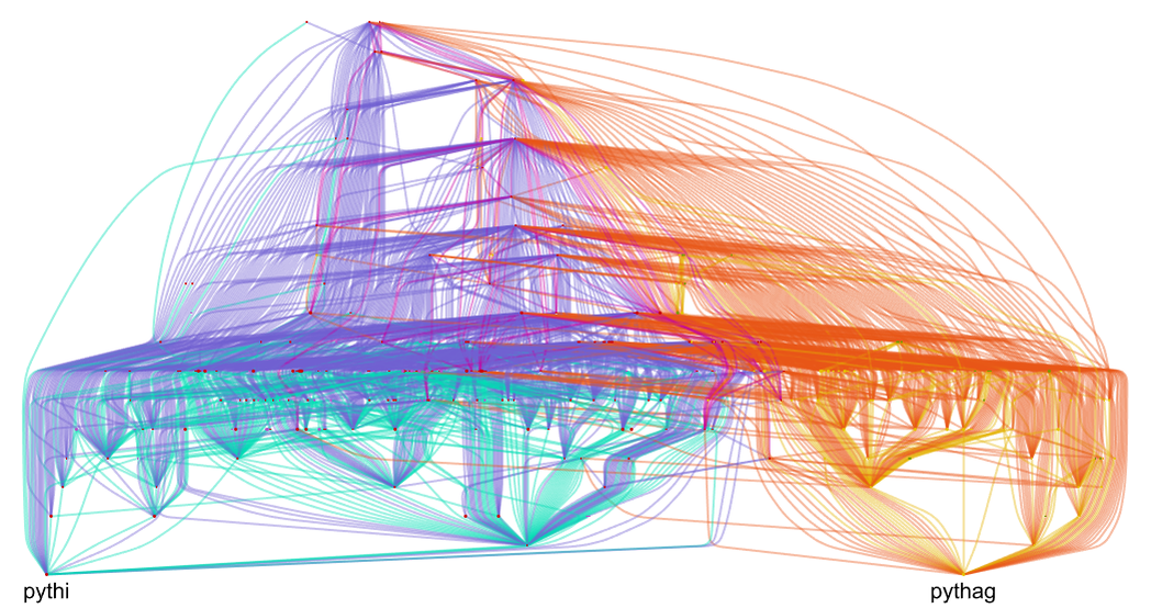
And what we see is there’s a certain amount of “lower-level overlap” between the derivations of these variants of the Pythagorean theorem, but also some discrepancy—indicating a certain separation between these variants in metamathematical space.
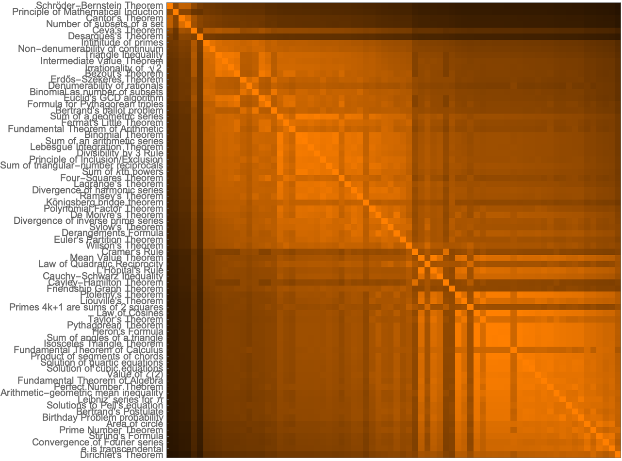
So what about other theorems? Here’s a table of some famous theorems from all over mathematics, sorted by the total number of theorems on which proofs of them formulated in Metamath depend—giving also the number of axioms and definitions used in each case:
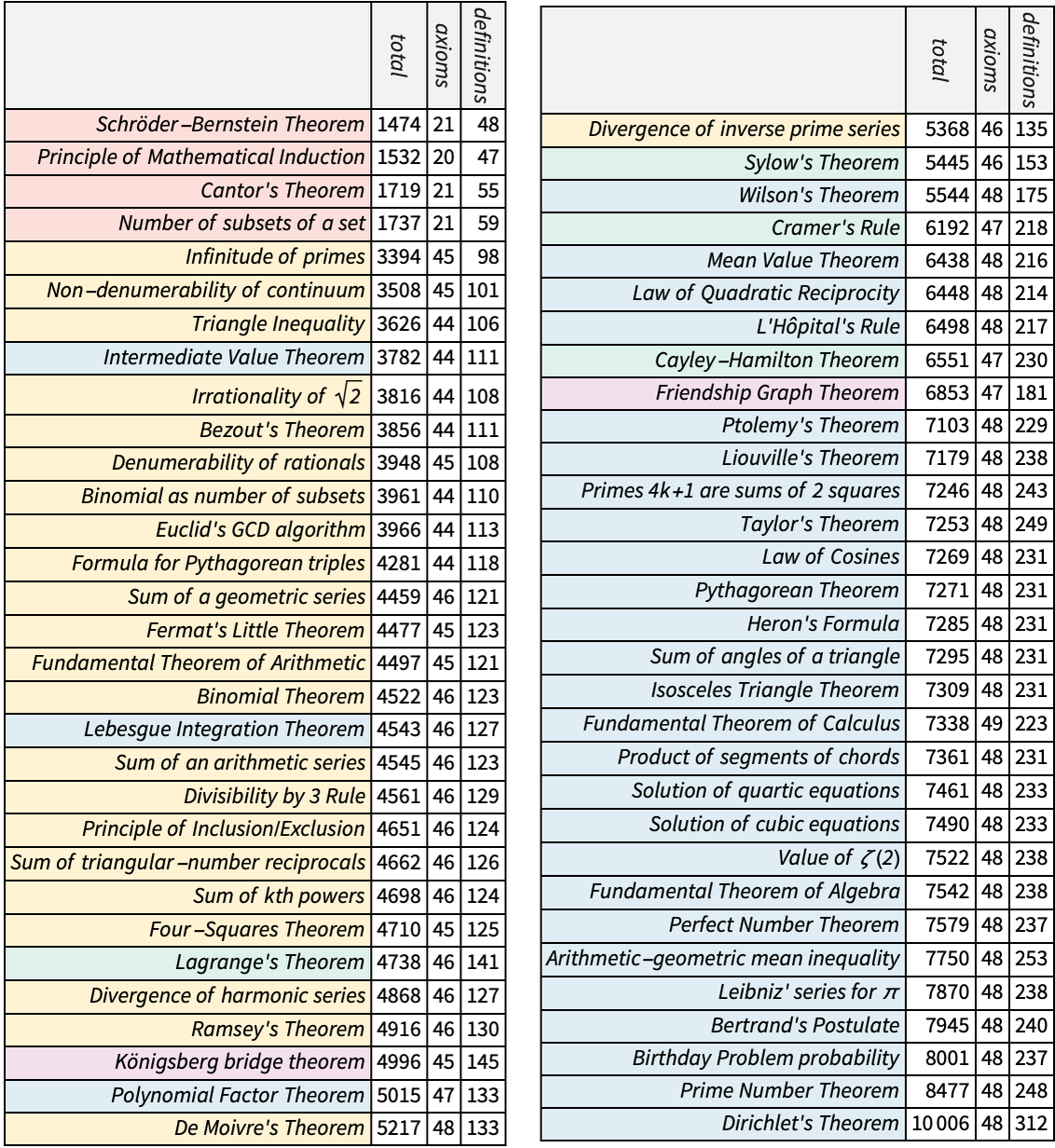
The Pythagorean theorem (here the pythi formulation) occurs solidly in the second half. Some of the theorems with the fewest dependencies are in a sense very structural theorems. But it’s interesting to see that theorems from all sorts of different areas soon start appearing, and then are very much mixed together in the remainder of the list. One might have thought that theorems involving “more sophisticated concepts” (like Ramsey’s theorem) would appear later than “more elementary” ones (like the sum of angles of a triangle). But this doesn’t seem to be true.
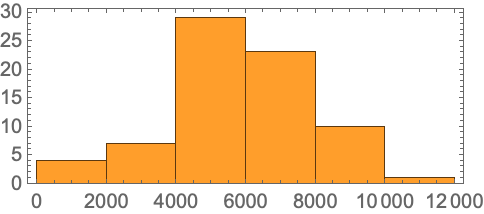
There’s a distribution of what amount to “proof sizes” (or, more strictly, theorem dependency sizes)—from the Schröder–Bernstein theorem which relies on less than 4% of all theorems, to Dirichlet’s theorem that relies on 25%:
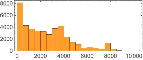
If we look not at “famous” theorems, but at all theorems covered by Metamath, the distribution becomes broader, with many short-to-prove “glue” or essentially “definitional” lemmas appearing:
But using the list of famous theorems as an indication of the “math that mathematicians care about” we can conclude that there is a kind of “metamathematical floor” of results that one needs to reach before “things that we care about” start appearing. It’s a bit like the situation in our Physics Project—where the vast majority of microscopic events that happen in the universe seem to be devoted merely to knitting together the structure of space, and only “on top of that” can events which can be identified with things like particles and motion appear.
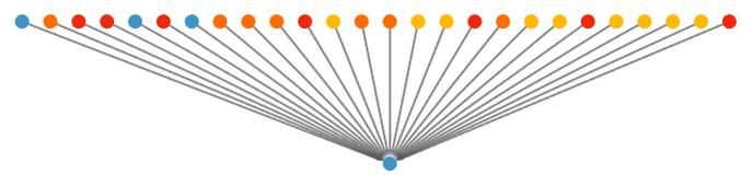
And indeed if we look at the “prerequisites” for different famous theorems, we indeed find that there is a large overlap (indicated by lighter colors)—supporting the impression that in a sense one first has “knit together metamathematical space” and only then can one start generating “interesting theorems”:
Another way to see “underlying overlap” is to look at what axioms different theorems ultimately depend on (the colors indicate the “depth” at which the axioms are reached):
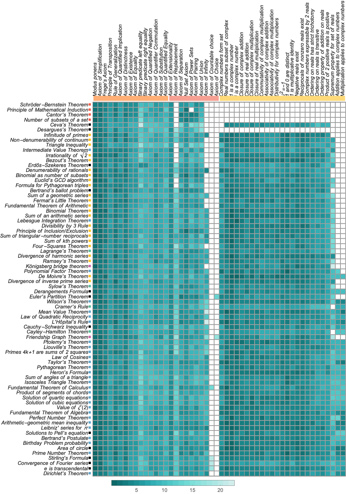
The theorems here are again sorted in order of “dependency size”. The “very-set-theoretic” ones at the top don’t depend on any of the various number-related axioms. And quite a few “integer-related theorems” don’t depend on complex number axioms. But otherwise, we see that (at least according to the proofs in set.mm) most of the “famous theorems” depend on almost all the axioms. The only axiom that’s rarely used is the Axiom of Choice—on which only things like “analysis-related theorems” such as the Fundamental Theorem of Calculus depend.
If we look at the “depth of proof” at which axioms are reached, there’s a definite distribution:
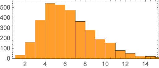
And this may be about as robust as any a “statistical characteristic” of the sampling of metamathematical space corresponding to mathematics that is “important to humans”. If we were, for example, to consider all possible theorems in the entailment cone we’d get a very different picture. But potentially what we see here may be a characteristic signature of what’s important to a “mathematical observer like us”.
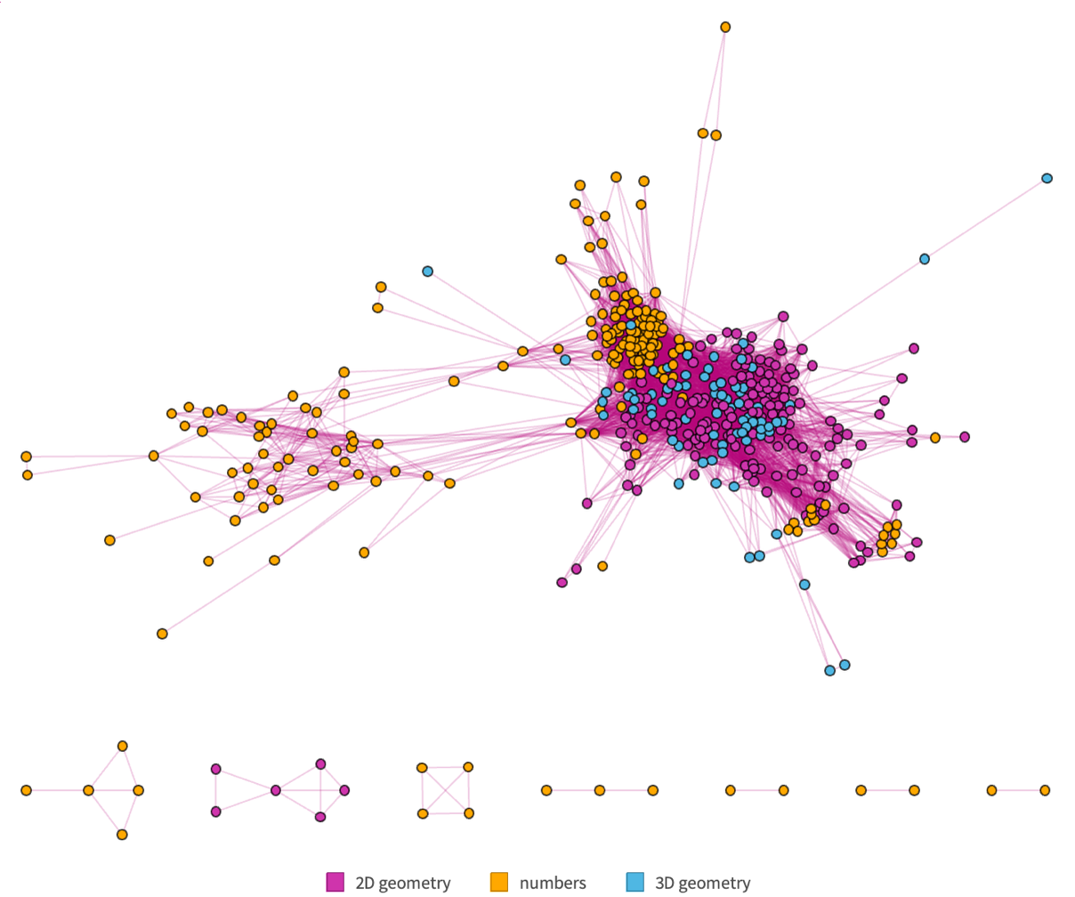
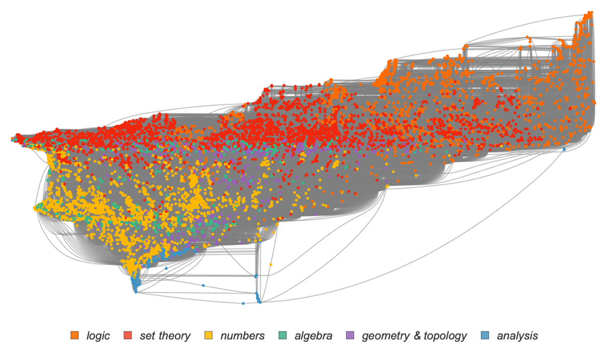
Going beyond “famous theorems” we can ask, for example, about all the 42,000 or so identified theorems in the Metamath set.mm collection. Here’s a rough rendering of their theorem dependency graph, with different colors indicating theorems in different fields of math (and with explicit edges removed):
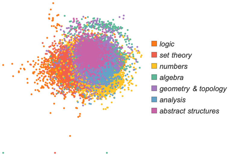
There’s some evidence of a certain overall uniformity, but we can see definite “patches of metamathematical space” dominated by different areas of mathematics. And here’s what happens if we zoom in on the central region, and show where famous theorems lie:
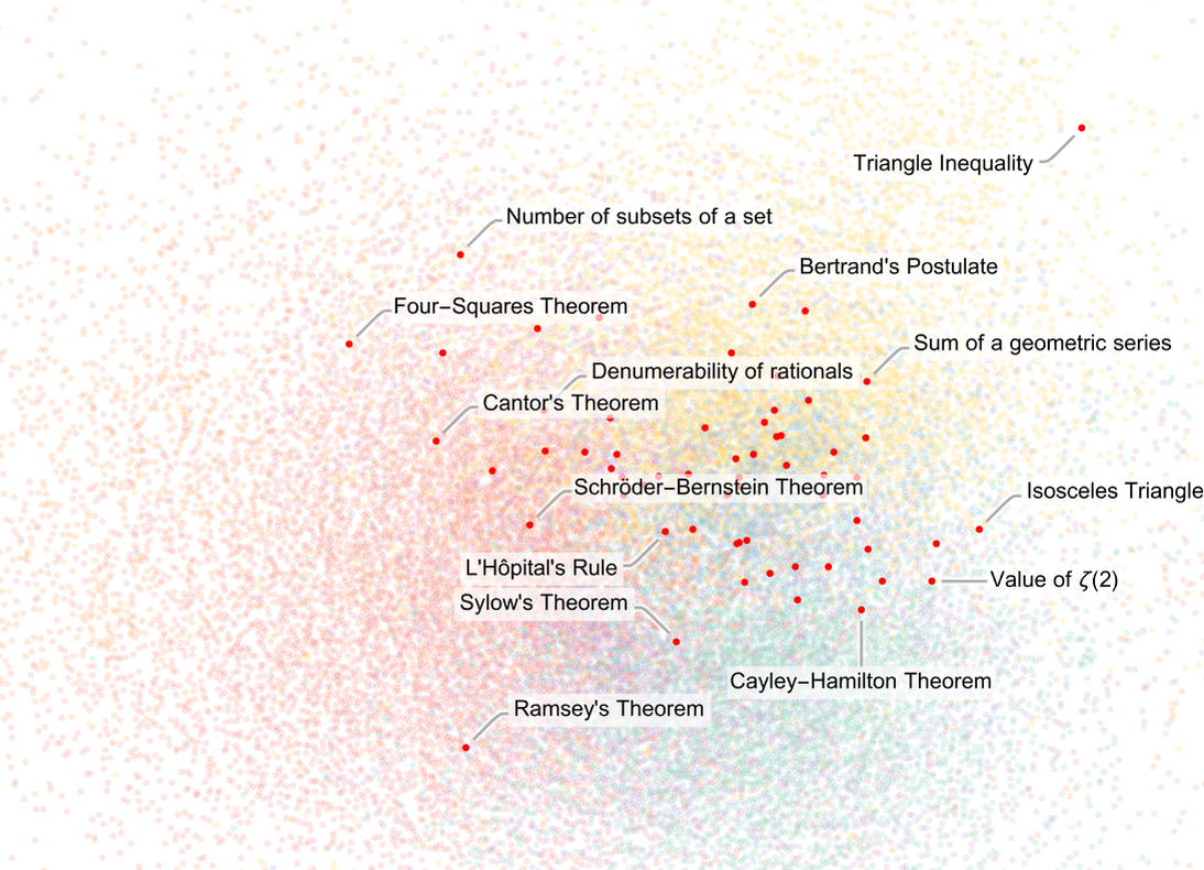
A bit like we saw for the named theorems of Boolean algebra clumps of famous theorems appear to somehow “stake out their own separate metamathematical territory”. But notably the famous theorems seem to show some tendency to congregate near “borders” between different areas of mathematics.
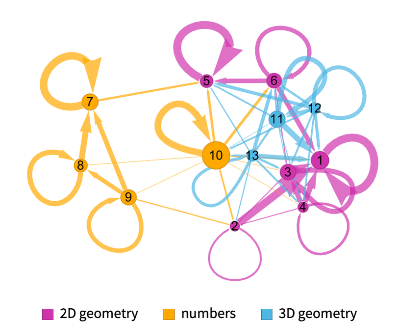
To get more of a sense of the relation between these different areas, we can make what amounts to a highly coarsened branchial graph, effectively laying out whole areas of mathematics in metamathematical space, and indicating their cross-connections:
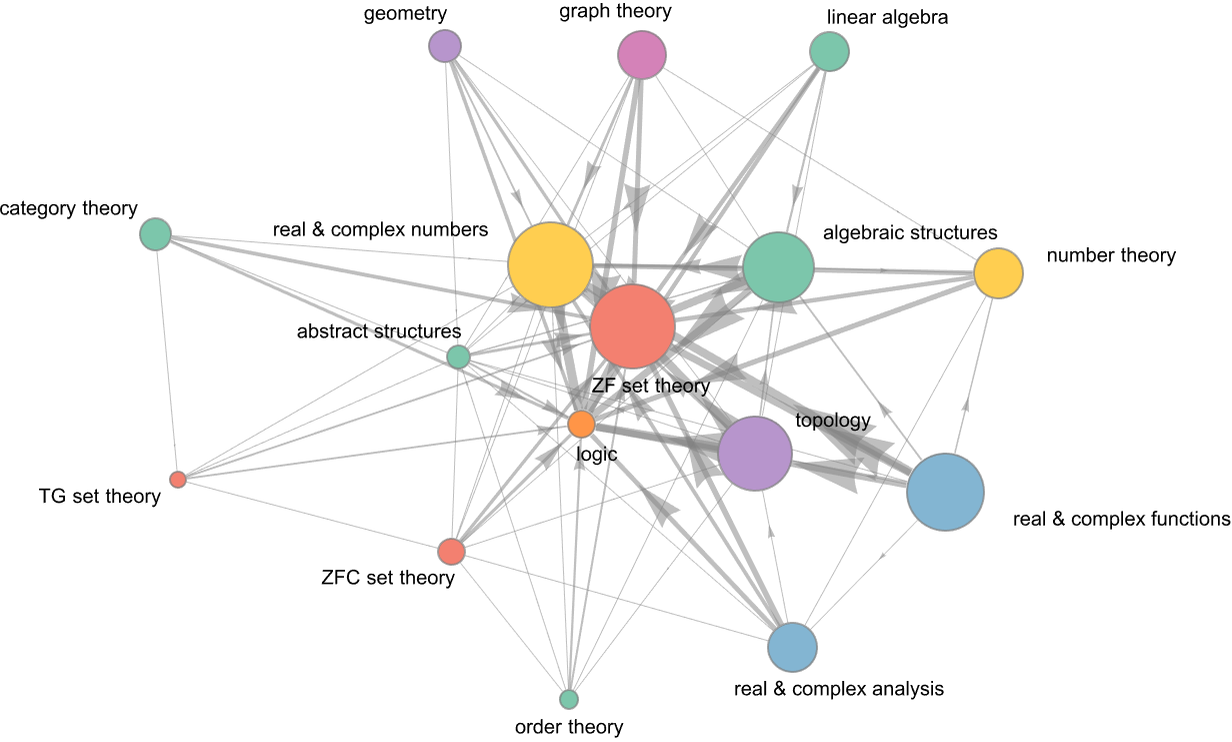
We can see “highways” between certain areas. But there’s also a definite “background entanglement” between areas, reflecting at least a certain background uniformity in metamathematical space, as sampled with the theorems identified in Metamath.
It’s not the case that all these areas of math “look the same”—and for example there are differences in their distributions of theorem dependency sizes:
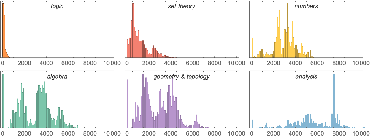
In areas like algebra and number theory, most proofs are fairly long, as revealed by the fact that they have many dependencies. But in set theory there are plenty of short proofs, and in logic all the proofs of theorems that have been included in Metamath are short.
What if we look at the overall dependency graph for all theorems in Metamath? Here's the adjacency matrix we get:
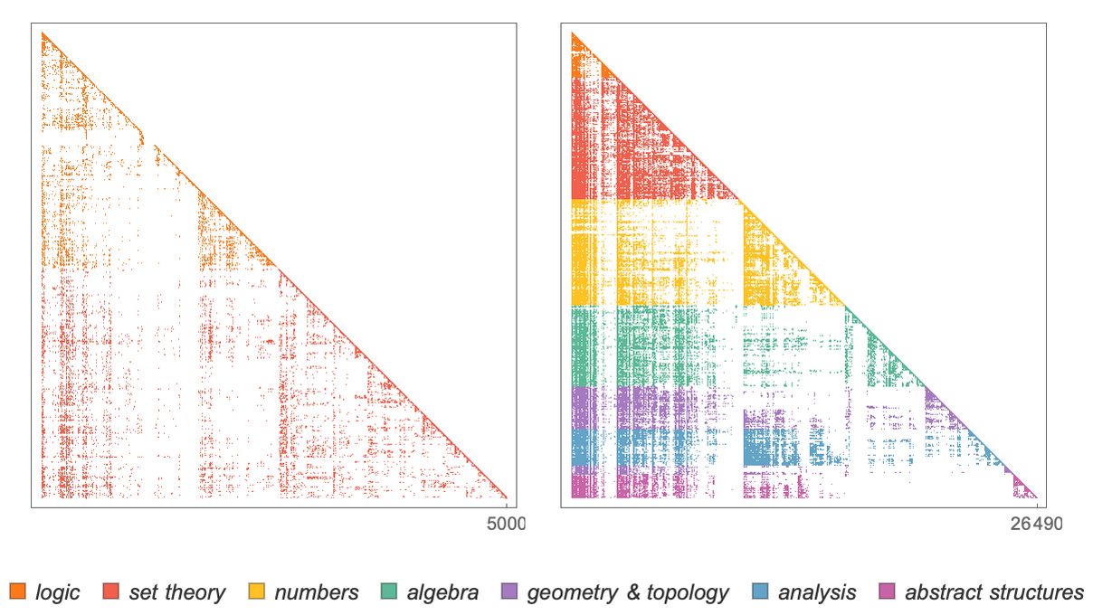
The results are triangular because theorems in the Metamath database are arranged so that later ones only depend on earlier ones. And while there’s considerable patchiness visible, there still seems to be a certain overall background level of uniformity.
In doing this empirical metamathematics we’re sampling metamathematical space just through particular “human mathematical settlements” in it. But even from the distribution of these “settlements” we potentially begin to see evidence of a certain background uniformity in metamathematical space.
Perhaps in time as more connections between different areas of mathematics are found human mathematics will gradually become more “uniformly settled” in metamathematical space—and closer to what we might expect from entailment cones and ultimately from the raw ruliad. But it’s interesting to see that even with fairly basic empirical metamathematics—operating on a current corpus of human mathematical knowledge—it may already be possible to see signs of some features of physicalized metamathematics.
One day, no doubt, we’ll be able do experiments in physics that take our “parsing” of the physical universe in terms of things like space and time and quantum mechanics—and reveal “slices” of the raw ruliad underneath. But perhaps something similar will also be possible in empirical metamathematics: to construct what amounts to a metamathematical microscope (or telescope) through which we can see aspects of the ruliad.