Consider all the mathematical statements that have appeared in mathematical books and papers. We can view these in some sense as the “observed phenomena” of (human) mathematics. And if we’re going to make a “general theory of mathematics” a first step is to do something like we’d typically do in natural science, and try to “drill down” to find a uniform underlying model—or at least representation—for all of them.
At the outset, it might not be clear what sort of representation could possibly capture all those different mathematical statements. But what’s emerged over the past century or so—with particular clarity in Mathematica and the Wolfram Language—is that there is in fact a rather simple and general representation that works remarkably well: a representation in which everything is a symbolic expression.
One can view a symbolic expression such as f[g[x][y, h[z]], w] as a hierarchical or tree structure, in which at every level some particular “head” (like f) is “applied to” one or more arguments. Often in practice one deals with expressions in which the heads have “known meanings”—as in Times[Plus[2, 3], 4] in Wolfram Language. And with this kind of setup symbolic expressions are reminiscent of human natural language, with the heads basically corresponding to “known words” in the language.
And presumably it’s this familiarity from human natural language that’s caused “human natural mathematics” to develop in a way that can so readily be represented by symbolic expressions.
But in typical mathematics there’s an important wrinkle. One often wants to make statements not just about particular things but about whole classes of things. And it’s common to then just declare that some of the “symbols” (like, say, x) that appear in an expression are “variables”, while others (like, say, Plus) are not. But in our effort to capture the essence of mathematics as uniformly as possible it seems much better to burn the idea of an object representing a whole class of things right into the structure of the symbolic expression.
And indeed this is a core idea in the Wolfram Language, where something like x or f is just a “symbol that stands for itself”, while x_ is a pattern (named x) that can stand for anything. (More precisely, _ on its own is what stands for “anything”, and x_—which can also be written x:_—just says that whatever _ stands for in a particular instance will be called x.)
Then with this notation an example of a “mathematical statement” might be:
In more explicit form we could write this as Equal[f[x_, y_], f[f[y_, x_],y_]]—where Equal () has the “known meaning” of representing equality. But what can we do with this statement? At a “mathematical level” the statement asserts that x_∘y_ and (y_∘x_)∘y_ should be considered equivalent. But thinking in terms of symbolic expressions there’s now a more explicit, lower-level, “structural” interpretation: that any expression whose structure matches x_∘y_ can equivalently be replaced by (y_∘x_)∘y_ (or, in Wolfram Language notation, just (y ∘ x) ∘ y) and vice versa. We can indicate this interpretation using the notation
which can be viewed as a shorthand for the pair of Wolfram Language rules:
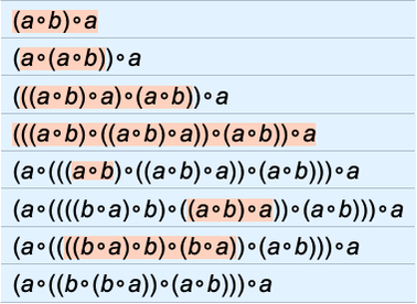
OK, so let’s say we have the expression (a∘b)∘a. Now we can just apply the rules defined by our statement. Here’s what happens if we do this just once in all possible ways:
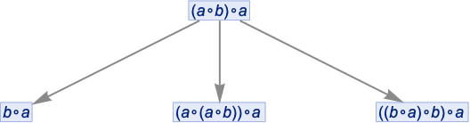
And here we see, for example, that (a∘b)∘a can be transformed to b∘a. Continuing this we build up a whole multiway graph. After just one more step we get:
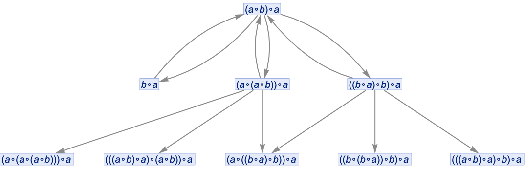
Continuing for a few more steps we then get
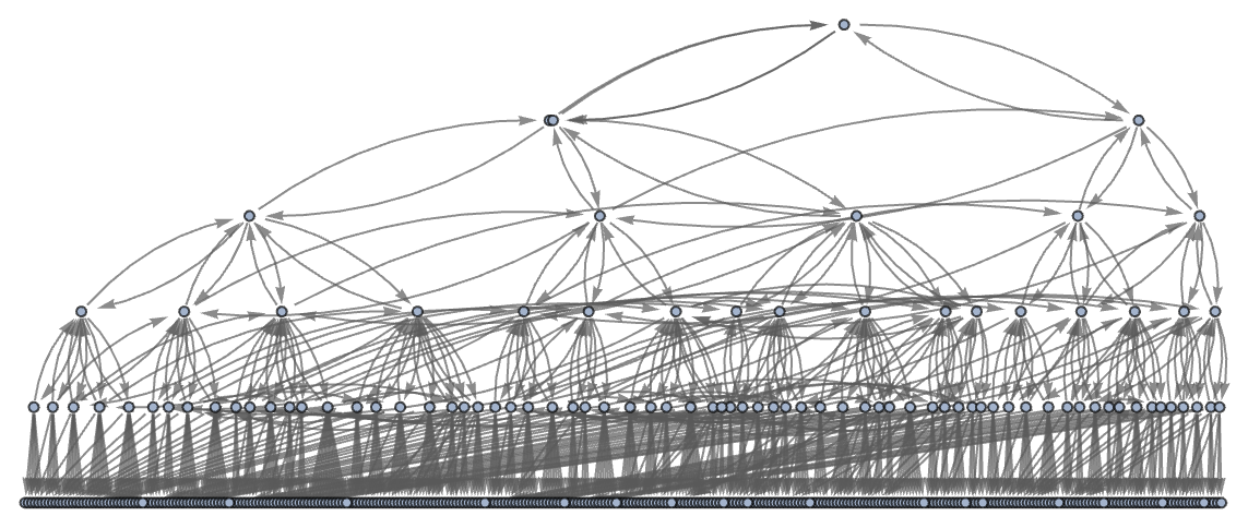
or in a different rendering:
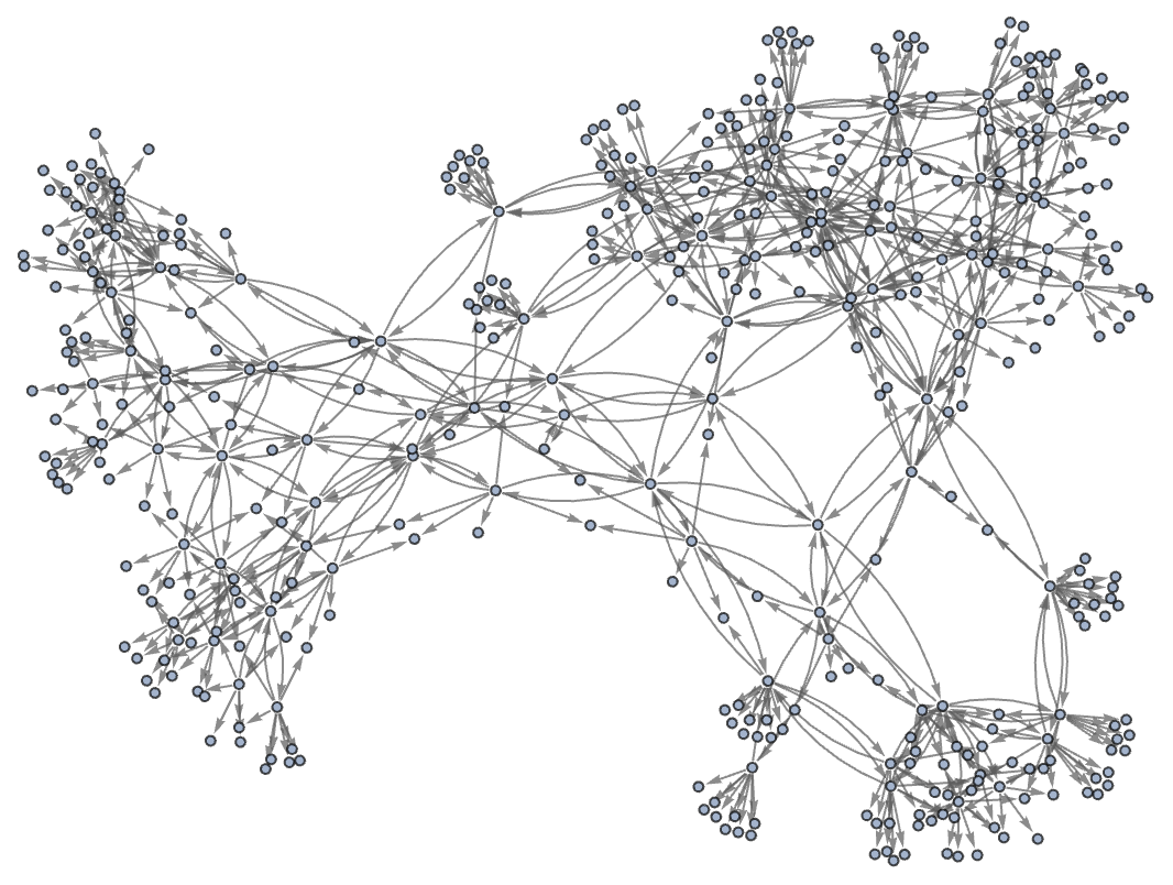
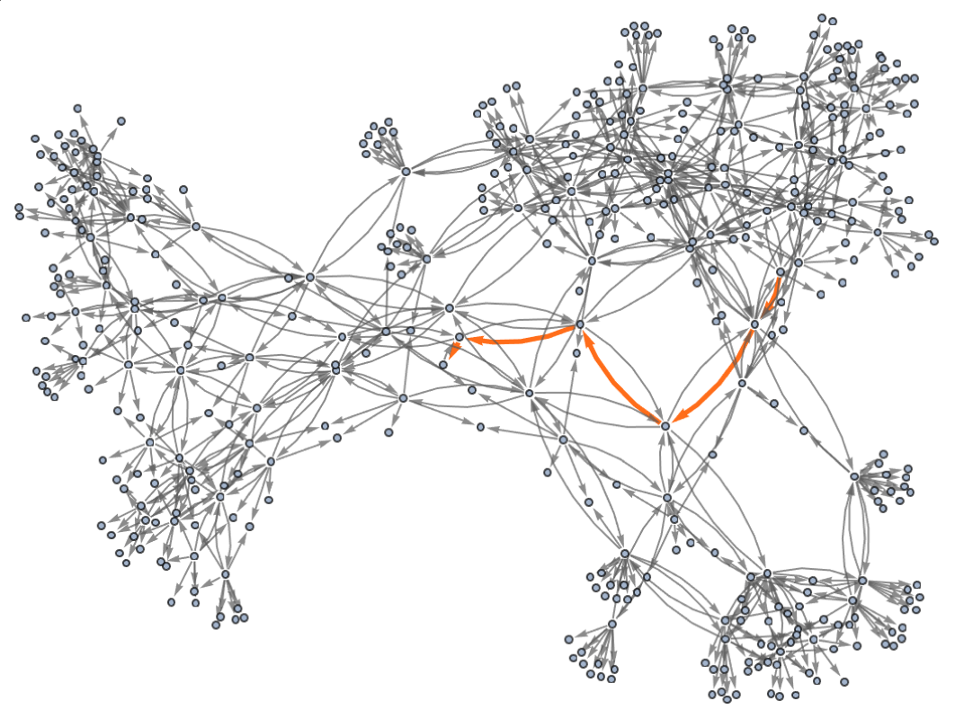
But what does this graph mean? Essentially it gives us a map of equivalences between expressions—with any pair of expressions that are connected being equivalent. So, for example, it turns out that the expressions (a∘((b∘a)∘(a∘b)))∘a and b∘a are equivalent, and we can “prove this” by exhibiting a path between them in the graph:
The steps on the path can then be viewed as steps in the proof, where here at each step we’ve indicated where the transformation in the expression took place:
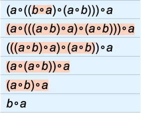
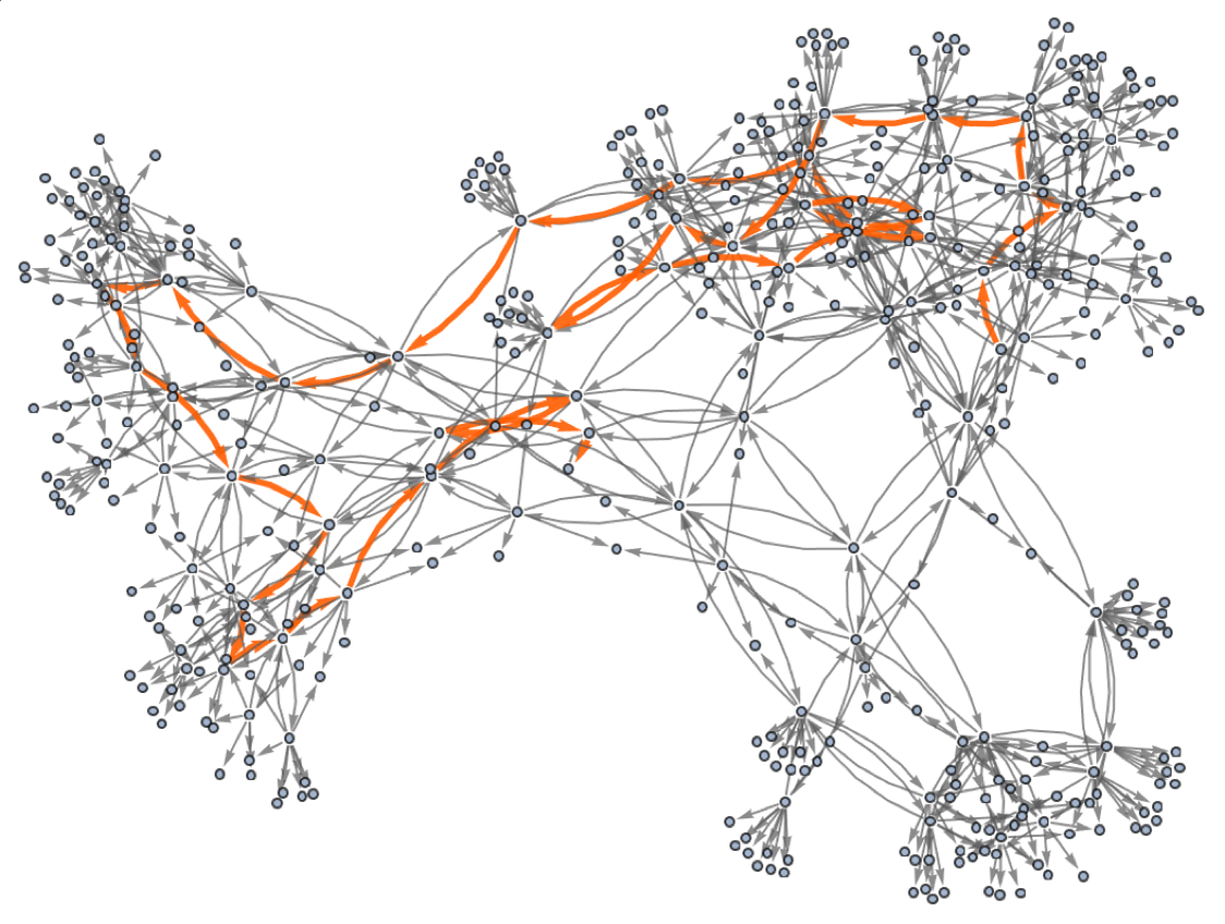
In mathematical terms, we can then say that starting from the “axiom” x∘y(y∘x)∘y we were able to prove a certain equivalence theorem between two expressions. We gave a particular proof. But there are others, for example the “less efficient” 35-step one
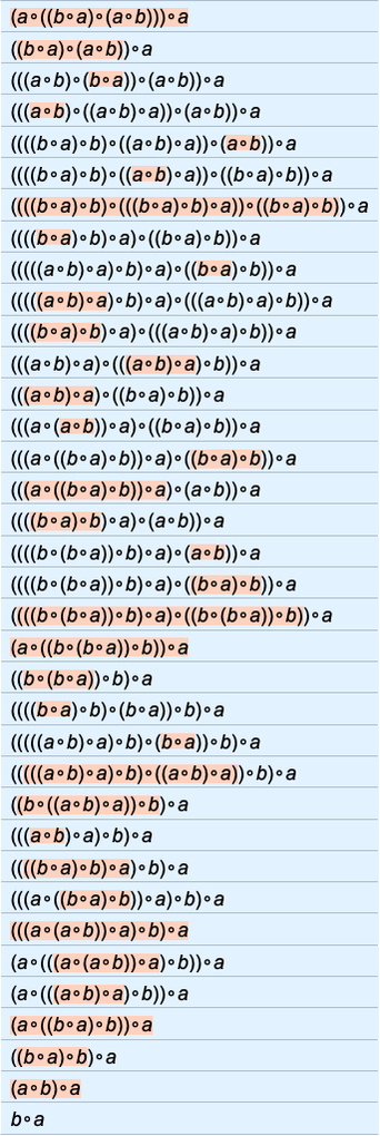
corresponding to the path:
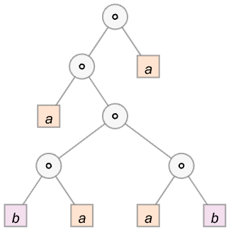
For our later purposes it’s worth talking in a little bit more detail here about how the steps in these proofs actually proceed. Consider the expression:
We can think of this as a tree:
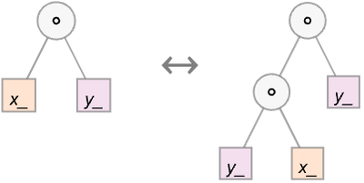
Our axiom can then be represented as:
In terms of trees, our first proof becomes
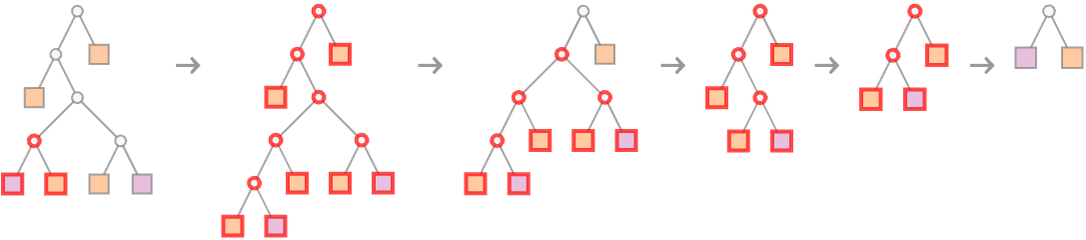
where we’re indicating at each step which piece of tree gets “substituted for” using the axiom.
What we’ve done so far is to generate a multiway graph for a certain number of steps, and then to see if we can find a “proof path” in it for some particular statement. But what if we are given a statement, and asked whether it can be proved within the specified axiom system? In effect this asks whether if we make a sufficiently large multiway graph we can find a path of any length that corresponds to the statement.
If our system was computationally reducible we could expect always to be able to find a finite answer to this question. But in general—with the Principle of Computational Equivalence and the ubiquitous presence of computational irreducibility—it’ll be common that there is no fundamentally better way to determine whether a path exists than effectively to try explicitly generating it. If we knew, for example, that the intermediate expressions generated always remained of bounded length, then this would still be a bounded problem. But in general the expressions can grow to any size—with the result that there is no general upper bound on the length of path necessary to prove even a statement about equivalence between small expressions.
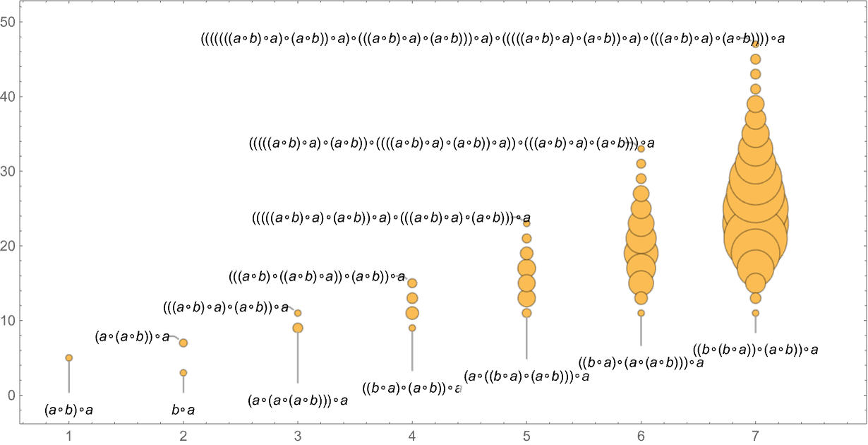
For example, for the axiom we are using here, we can look at statements of the form (a∘b)∘aexpr. Then this shows how many expressions expr of what sizes have shortest proofs of (a∘b)∘aexpr with progressively greater lengths:
And for example if we look at the statement
its shortest proof is
where, as is often the case, there are intermediate expressions that are longer than the final result.